Standard Deviation of Continuous Series
A continuous series groups data into classes such as 0-10, 10-20 and 20-30, and records how many items fall in each class. Once data is grouped like this, we no longer know the exact value of each item. A salary of Rs. 13,000 and a salary of Rs. 19,000 both sit inside the class 10-20 (in thousands), and the table does not tell them apart. We still want to know how spread out the data is, and the standard deviation still measures that. The only change is that every class must first be represented by one number.
Standard deviation \( (\sigma) \): the positive square root of the mean of the squared deviations of the values from their arithmetic mean. It measures dispersion. A small standard deviation means the values crowd close to the mean; a large one means they are widely spread.
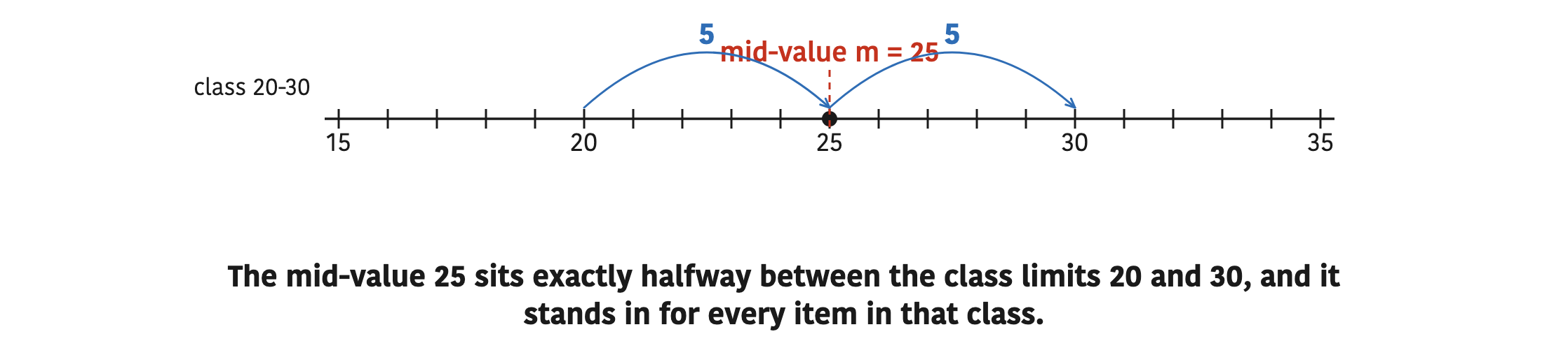
Mid-value \( (m) \): the middle point of a class interval, found by adding the lower and upper limits and dividing by 2. It stands for every item in that class.
\[ m = \frac{\text{lower limit} + \text{upper limit}}{2} \]
For the class 20-30, the mid-value is \( m = \frac{20 + 30}{2} = 25 \). Every student who scored somewhere from 20 up to 30 is treated as if they scored 25.
In every method below, \( N \) is the sum of the frequencies, \( N = \sum f \), and the mid-values \( m \) take the place of the unknown individual values. There are four methods. All four give the same standard deviation. They differ only in how heavy the arithmetic is, so the skill is choosing the one that keeps your numbers small.
- Actual mean method: deviations are measured from the true mean.
- Direct method: the mid-values are used as they are, with no mean subtracted.
- Short-cut method or assumed mean method: deviations are measured from a convenient assumed mean.
- Step deviation method: deviations from the assumed mean are divided by the class width to make them tiny.
Actual Mean Method
In this method we first calculate the actual mean of the data. Then we measure how far each mid-value lies from that mean, square each distance, weight it by its frequency, find the average and take the square root. This is formula (i):
\[ \sigma = \sqrt{\frac{\sum f(m - \bar{X})^2}{N}} \]
Here \( m \) is the mid-value, \( N \) is the sum of the frequencies and \( \bar{X} \) is the mean, found as \( \bar{X} = \frac{\sum fm}{N} \). The method follows these steps:
- (a) Find the mid-value \( m \) of each class.
- (b) Multiply each frequency \( f \) by its mid-value to get \( fm \), and add these to get \( \sum fm \).
- (c) Find the mean \( \bar{X} = \frac{\sum fm}{N} \).
- (d) Subtract \( \bar{X} \) from each \( m \) and square the answer to get \( (m - \bar{X})^2 \).
- (e) Multiply each \( (m - \bar{X})^2 \) by its frequency to get \( f(m - \bar{X})^2 \).
- (f) Add these to get \( \sum f(m - \bar{X})^2 \).
- (g) Put the totals into formula (i).
Example 1. The monthly salaries of 100 employees of a company are given below, in thousands of rupees. Find the standard deviation by the actual mean method, and its coefficient.
| Salary (Rs. in thousand) | 0-10 | 10-20 | 20-30 | 30-40 | 40-50 | 50-60 |
| Number of employees | 8 | 12 | 20 | 40 | 12 | 8 |
Step 1: The mid-values are 5, 15, 25, 35, 45 and 55. Multiplying each by its frequency and adding gives \( \sum fm = 3100 \), with \( N = 100 \). So the mean is:
\[ \bar{X} = \frac{\sum fm}{N} = \frac{3100}{100} = 31 \]
Step 2: Since the mean is 31, each deviation is \( m - 31 \). Squaring each deviation and multiplying by its frequency gives this working table:
| Salary | f | m | fm | \( (m - 31)^2 \) | \( f(m - 31)^2 \) |
| 0-10 | 8 | 5 | 40 | 676 | 5408 |
| 10-20 | 12 | 15 | 180 | 256 | 3072 |
| 20-30 | 20 | 25 | 500 | 36 | 720 |
| 30-40 | 40 | 35 | 1400 | 16 | 640 |
| 40-50 | 12 | 45 | 540 | 196 | 2352 |
| 50-60 | 8 | 55 | 440 | 576 | 4608 |
| Total | N = 100 | \( \sum fm = 3100 \) | 16800 |
Step 3: Substituting \( \sum f(m - \bar{X})^2 = 16800 \) and \( N = 100 \) into formula (i):
\[ \sigma = \sqrt{\frac{16800}{100}} \]
Step 4: Dividing, then taking the square root:
\[ \sigma = \sqrt{168} = 12.96 \]
So the standard deviation of the salaries is 12.96 thousand rupees. A second number tells us how large this spread is compared with the mean.
Coefficient of standard deviation: the standard deviation divided by the mean, \( \frac{\sigma}{\bar{X}} \). It has no unit, so it can compare the spread of two sets measured in different units or around very different means.
Step 5: Dividing the standard deviation by the mean gives the coefficient:
\[ \frac{\sigma}{\bar{X}} = \frac{12.96}{31} = 0.418 \]
Therefore \( \sigma = 12.96 \) and its coefficient is 0.418. The actual mean method is comfortable here because the mean came out as the whole number 31. If the mean had been 31.47, every deviation would have been a messy decimal, and one of the next three methods would be wiser.
Direct Method
The direct method uses neither the actual mean nor an assumed mean. The mid-values are used straight away, together with their squares. It suits data whose mid-values are small numbers, because then the squares stay manageable. This is formula (ii):
\[ \sigma = \sqrt{\frac{\sum fm^2}{N} - \left(\frac{\sum fm}{N}\right)^2} \]
Here \( m \) is the mid-value and \( N \) is the sum of the frequencies. The term \( fm^2 \) means \( f \times m^2 \). The quickest way to get it is to multiply the \( fm \) column by \( m \) once more.
\( fm^2 \) is \( f \times m \times m \), not \( (f \times m)^2 \). For \( f = 3 \) and \( m = 5 \), \( fm^2 = 75 \), but \( (fm)^2 = 225 \). Squaring the whole product makes every answer far too large.
- (a) Find the mid-value \( m \) of each class.
- (b) Multiply each \( f \) by its \( m \) to get \( fm \).
- (c) Multiply each \( fm \) by its \( m \) again to get \( fm^2 \).
- (d) Add the columns to get \( \sum fm \) and \( \sum fm^2 \).
- (e) Put the totals into formula (ii).
Example 2. The marks obtained by 20 students are given below. Find the standard deviation by the direct method.
| Marks obtained | 0-10 | 10-20 | 20-30 | 30-40 | 40-50 |
| Number of students | 3 | 5 | 7 | 3 | 2 |
Step 1: The mid-values, the products \( fm \) and the products \( fm^2 \) are worked out in a table:
| Marks | f | m | fm | \( fm^2 \) |
| 0-10 | 3 | 5 | 15 | 75 |
| 10-20 | 5 | 15 | 75 | 1125 |
| 20-30 | 7 | 25 | 175 | 4375 |
| 30-40 | 3 | 35 | 105 | 3675 |
| 40-50 | 2 | 45 | 90 | 4050 |
| Total | N = 20 | 460 | 13300 |
Step 2: Substituting \( N = 20 \), \( \sum fm = 460 \) and \( \sum fm^2 = 13300 \) into formula (ii):
\[ \sigma = \sqrt{\frac{13300}{20} - \left(\frac{460}{20}\right)^2} \]
Step 3: Dividing inside the root. Since \( \frac{13300}{20} = 665 \) and \( \frac{460}{20} = 23 \), this becomes:
\[ \sigma = \sqrt{665 - 23^2} = \sqrt{665 - 529} \]
Step 4: Subtracting and taking the square root:
\[ \sigma = \sqrt{136} = 11.66 \]
So the standard deviation of the marks is 11.66.
Look again at formula (ii). The fraction \( \frac{\sum fm}{N} \) is simply the mean, which was 23 in Example 2. So the direct method says: take the mean of the squares, subtract the square of the mean, then take the square root.
Short-cut Method or Assumed Mean Method
When the actual mean comes out as an awkward decimal, subtracting it from every mid-value is slow and easy to get wrong. Instead, we pick a convenient mid-value near the middle of the table and treat it as if it were the mean. Deviations measured from it are small whole numbers. The formula then corrects for the fact that this value is not the true mean.
Assumed mean \( (A) \): a convenient value, usually the middle mid-value of the table, used in place of the actual mean so that the deviations \( d = m - A \) are easy to work with.
This is formula (iii):
\[ \sigma = \sqrt{\frac{\sum fd^2}{N} - \left(\frac{\sum fd}{N}\right)^2} \]
Here \( d = m - A \), \( m \) is the mid-value, \( N \) is the sum of the frequencies and \( A \) is the assumed mean. The steps are:
- (a) Find the mid-value \( m \) of each class.
- (b) Take the middle mid-value as the assumed mean \( A \), and find each deviation \( d = m - A \).
- (c) Multiply each \( d \) by its frequency to get \( fd \).
- (d) Multiply each \( fd \) by its \( d \) again to get \( fd^2 \).
- (e) Add the columns to get \( \sum fd \) and \( \sum fd^2 \).
- (f) Put the totals into formula (iii).
Example 3. The marks of 60 students are given below. Find the standard deviation by the short-cut method.
| Marks obtained | 20-30 | 30-40 | 40-50 | 50-60 | 60-70 |
| Number of students | 10 | 15 | 20 | 8 | 7 |
Step 1: The mid-values are 25, 35, 45, 55 and 65. The middle one, 45, is taken as the assumed mean, so \( d = m - 45 \). The working table is:
| Marks | f | m | \( d = m - 45 \) | fd | \( fd^2 \) |
| 20-30 | 10 | 25 | -20 | -200 | 4000 |
| 30-40 | 15 | 35 | -10 | -150 | 1500 |
| 40-50 | 20 | 45 (A) | 0 | 0 | 0 |
| 50-60 | 8 | 55 | 10 | 80 | 800 |
| 60-70 | 7 | 65 | 20 | 140 | 2800 |
| Total | N = 60 | -130 | 9100 |
Step 2: Substituting \( N = 60 \), \( \sum fd = -130 \) and \( \sum fd^2 = 9100 \) into formula (iii):
\[ \sigma = \sqrt{\frac{9100}{60} - \left(\frac{-130}{60}\right)^2} \]
Step 3: Dividing inside the root. Since \( \frac{9100}{60} = 151.67 \) and \( \frac{-130}{60} = -2.167 \), whose square is 4.694, this becomes:
\[ \sigma = \sqrt{151.67 - 4.694} \]
Step 4: Subtracting and taking the square root:
\[ \sigma = \sqrt{146.97} = 12.12 \]
So the standard deviation of the marks is 12.12. Notice that we never had to find the actual mean to get this answer.
A negative deviation keeps its sign in the \( fd \) column, but \( fd^2 = fd \times d \) is always positive, because a negative times a negative is positive. In the same way \( \left(\frac{-130}{60}\right)^2 \) is positive, so the formula always subtracts a positive number.
Step Deviation Method
Suppose the mid-values are large, such as 50, 150, 250, 350 and 450. Even after subtracting an assumed mean of 250, the deviations are -200, -100, 0, 100 and 200, and their squares run into tens of thousands. When all the classes have the same width, every one of these deviations is a multiple of that width. Dividing by the width shrinks them to -2, -1, 0, 1 and 2. We work with these tiny numbers and multiply back by the width at the very end.
Step deviation \( (d') \): the deviation of a mid-value from the assumed mean, divided by the class width \( h \). So \( d' = \frac{d}{h} = \frac{m - A}{h} \).
This is formula (iv):
\[ \sigma = \sqrt{\frac{\sum fd'^2}{N} - \left(\frac{\sum fd'}{N}\right)^2} \times h \]
Here \( m \) is the mid-value, \( N \) is the sum of the frequencies, \( h \) is the class width (the size of each class interval) and \( A \) is the assumed mean. The steps are:
- (a) Find the mid-value \( m \) of each class.
- (b) Take the middle mid-value as the assumed mean \( A \), subtract it from each mid-value and divide by the class width \( h \) to get \( d' \).
- (c) Multiply each \( d' \) by its frequency to get \( fd' \).
- (d) Multiply each \( fd' \) by its \( d' \) again to get \( fd'^2 \).
- (e) Add the columns to get \( \sum fd' \) and \( \sum fd'^2 \).
- (f) Put the totals into formula (iv), remembering the final multiplication by \( h \).
Example 4. The hourly wages of 25 workers are given below. Find the standard deviation by the step deviation method.
| Wage (Rs. per hour) | 0-100 | 100-200 | 200-300 | 300-400 | 400-500 |
| Number of workers | 5 | 8 | 7 | 3 | 2 |
Step 1: The mid-values are 50, 150, 250, 350 and 450. Taking \( A = 250 \) and \( h = 100 \) gives \( d' = \frac{m - 250}{100} \). The working table is:
| Wage | f | m | \( d' = \frac{m - 250}{100} \) | fd' | \( fd'^2 \) |
| 0-100 | 5 | 50 | -2 | -10 | 20 |
| 100-200 | 8 | 150 | -1 | -8 | 8 |
| 200-300 | 7 | 250 | 0 | 0 | 0 |
| 300-400 | 3 | 350 | 1 | 3 | 3 |
| 400-500 | 2 | 450 | 2 | 4 | 8 |
| Total | N = 25 | -11 | 39 |
Step 2: Substituting \( N = 25 \), \( \sum fd' = -11 \), \( \sum fd'^2 = 39 \) and \( h = 100 \) into formula (iv):
\[ \sigma = \sqrt{\frac{39}{25} - \left(\frac{-11}{25}\right)^2} \times 100 \]
Step 3: Dividing inside the root. Since \( \frac{39}{25} = 1.56 \) and \( \left(\frac{-11}{25}\right)^2 = (-0.44)^2 = 0.1936 \), this becomes:
\[ \sigma = \sqrt{1.56 - 0.1936} \times 100 \]
Step 4: Subtracting and taking the square root:
\[ \sigma = \sqrt{1.3664} \times 100 = 1.1689 \times 100 \]
Step 5: Multiplying by the class width:
\[ \sigma = 116.89 \]
So the standard deviation of the hourly wages is Rs. 116.89.
Do not stop at 1.1689. The square root gives the spread measured in class widths, and the last step multiplies by \( h \) to turn it back into rupees. Leaving out \( \times h \) gives an answer 100 times too small here.
Four methods, one answer. As a check, take the salary data of Example 1 again and use the step deviation method with \( A = 35 \) and \( h = 10 \). The step deviations are -3, -2, -1, 0, 1 and 2, which give \( \sum fd' = -40 \) and \( \sum fd'^2 = 184 \) with \( N = 100 \). Substituting into formula (iv):
\[ \sigma = \sqrt{\frac{184}{100} - \left(\frac{-40}{100}\right)^2} \times 10 \]
Simplifying inside the root, \( 1.84 - 0.16 = 1.68 \), so:
\[ \sigma = \sqrt{1.68} \times 10 = 12.96 \]
This is exactly the 12.96 found by the actual mean method. The method changes the arithmetic, never the answer. Choose the one that keeps your numbers smallest.
Choosing a Method
Before you start a question, look at the mid-values and ask which method will give the lightest working. The table below puts the four side by side.
| Method | Deviation used | Best when |
| Actual mean | \( m - \bar{X} \) | the mean is a whole number |
| Direct | \( m \) itself | the mid-values are small |
| Short-cut or assumed mean | \( d = m - A \) | the actual mean is a decimal |
| Step deviation | \( d' = \frac{m - A}{h} \) | the mid-values are large and the classes are equal in width |
If a question names the method, use that method, even if another would be quicker. The examiner is checking that you can carry out the method asked for.
Comparing Consistency with the Coefficient of Variation
Standard deviation is measured in the same units as the data. That makes it unfair for comparing two groups whose means are very different. A spread of Rs. 110 is huge for pocket money that averages Rs. 200, but tiny for a salary that averages Rs. 40,000. To compare fairly, we express the standard deviation as a percentage of the mean.
Coefficient of variation (C.V.): the standard deviation expressed as a percentage of the mean. The set with the smaller C.V. is more uniform, that is, more consistent; the set with the larger C.V. is more variable.
\[ \text{C.V.} = \frac{\sigma}{\bar{X}} \times 100\% \]
Variance: the square of the standard deviation, \( \sigma^2 \). If the variance is 64, the standard deviation is \( \sqrt{64} = 8 \).
Example 5. The salaries of the employees of two industries are analysed in the table below. Find which industry has more uniformity in its salary distribution.
| Industry | Average monthly salary | Standard deviation of salary |
| A | Rs. 50000 | Rs. 100 |
| B | Rs. 40000 | Rs. 110 |
Here the mean salary of industry A is \( \bar{X}_1 = 50000 \) and its standard deviation is \( \sigma_1 = 100 \). For industry B, \( \bar{X}_2 = 40000 \) and \( \sigma_2 = 110 \).
Step 1: Finding the coefficient of variation of industry A:
\[ \text{C.V.}_A = \frac{100}{50000} \times 100\% = 0.2\% \]
Step 2: Finding the coefficient of variation of industry B:
\[ \text{C.V.}_B = \frac{110}{40000} \times 100\% = 0.275\% \]
Step 3: Comparing the two. Since \( 0.2\% < 0.275\% \), industry A has the smaller coefficient of variation. So the salaries of industry A are more uniform than those of industry B.
Do not judge uniformity from the standard deviation alone. Group P has mean 20 and standard deviation 5, so its C.V. is 25%. Group Q has mean 200 and standard deviation 20, so its C.V. is 10%. Q has the bigger standard deviation, yet Q is the more uniform group, because its spread is small compared with its mean.
The full lesson is waiting for you
The notes are free to read in full. A free account opens the rest of the practice, and tracks your progress and confidence score for every subject. Presentations and videos need approval from Learn Yeti.