How Far Do the Values Lie from the Average?
An average tells us where the centre of a set of data is. It does not tell us how the values are spread around that centre. Sita scored 48, 50 and 52 marks in three tests. Hari scored 30, 50 and 70. Both have a mean of 50. Sita's marks sit close together, while Hari's are scattered far apart. If we reported only the mean, the two students would look exactly alike.
To tell them apart, we look at how far each mark lies from the mean. Sita's marks are 2, 0 and 2 marks away from 50. Hari's marks are 20, 0 and 20 marks away. Sita's average distance is \( \frac{2 + 0 + 2}{3} \approx 1.33 \) marks and Hari's is \( \frac{20 + 0 + 20}{3} \approx 13.33 \) marks. A small average distance means the data is packed tightly; a large one means it is spread out. This average distance is the idea behind mean deviation.
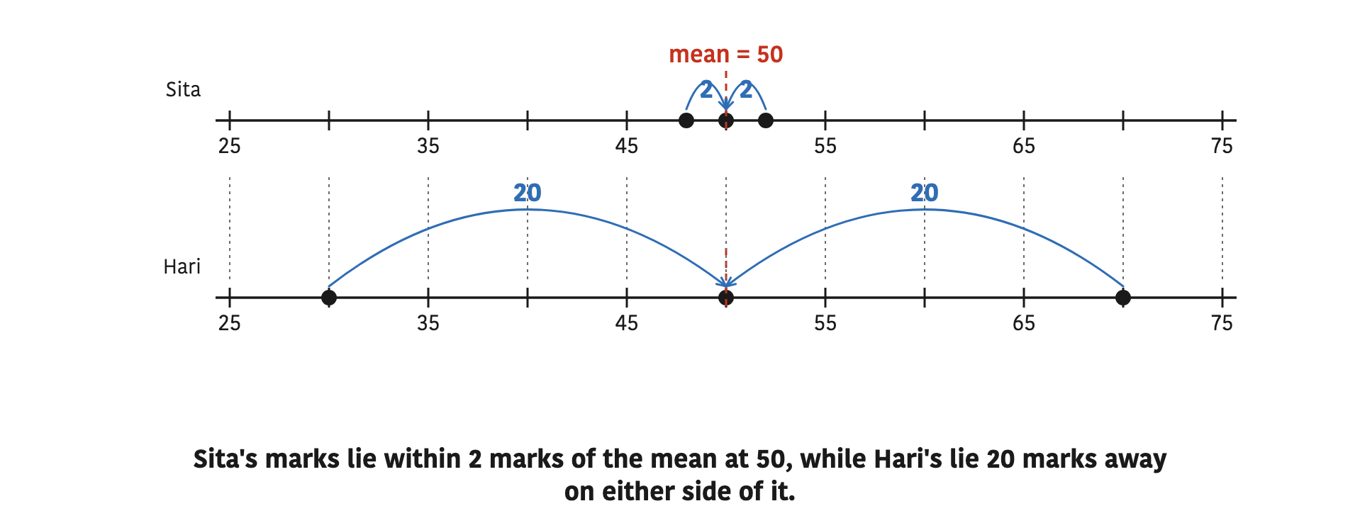
Why the Sign Is Dropped: Absolute Value
A deviation is found by subtracting the average from a value. For Hari, 30 - 50 = -20 and 70 - 50 = 20. A value below the mean gives a negative deviation and a value above it gives a positive one. If we simply added these, they would cancel: -20 + 0 + 20 = 0. Deviations taken from the mean always cancel out like this, so their plain average tells us nothing about the spread.
Deviation: the difference between a value and an average of the data. For grouped data we use the mid-value m of each class, so the deviation from the mean is \( D = m - \bar{X} \).
What we really want is a distance, and a distance is never negative. So every deviation is counted as positive, whatever its sign. Mathematics does this with the absolute value.
Absolute value: the size of a number without its sign, written between two vertical bars. So \( |-20| = 20 \) and \( |20| = 20 \).
Do not multiply and add the deviations D with their signs. Taken from the mean, \( \Sigma f(m - \bar{X}) \) comes to zero, or almost zero after rounding. Change each D into \( |D| \) first, and only then multiply by f.
Mean Deviation
Mean deviation (MD): the average of the absolute values of the differences between each item of the data and their mean or median.
Mean deviation is itself an average. It is the average distance of the items from a central value, and it shows how widely the data is spread. The central value can be any average: the mean, the median or the mode. That is why we speak of mean deviation from the mean and mean deviation from the median. At this level we calculate it from the mean and from the median.
Coefficient of mean deviation: the mean deviation divided by the average it was measured from. It is a pure number with no unit, and it is used to compare the spread of different sets of data.
Formulas for Mean Deviation
In grouped data each class is represented by its mid-value m, f is the frequency of the class and \( N = \Sigma f \) is the total frequency. \( \bar{X} \) stands for the mean and \( M_d \) for the median. There are four relations to know.
(a) Mean deviation from the mean:
\[ \text{MD} = \frac{\Sigma f|m - \bar{X}|}{N} = \frac{\Sigma f|D|}{N} \]
(b) Coefficient of mean deviation from the mean:
\[ \text{Coefficient} = \frac{\text{MD from mean}}{\text{Mean}} \]
(c) Mean deviation from the median:
\[ \text{MD} = \frac{\Sigma f|m - M_d|}{N} = \frac{\Sigma f|D|}{N} \]
(d) Coefficient of mean deviation from the median:
\[ \text{Coefficient} = \frac{\text{MD from median}}{\text{Median}} \]
The mean and the median that go into these formulas are found in the usual way for grouped data:
\[ \bar{X} = \frac{\Sigma fm}{N} \]
\[ M_d = L + \frac{\frac{N}{2} - cf}{f} \times i \]
In the median formula, L is the lower limit of the median class, cf is the cumulative frequency of the class just before it, f is the frequency of the median class and i is its class width.
Both mean deviation formulas have the same shape. Only the centre changes: \( |D| \) is measured from the mean in one and from the median in the other. The coefficient always divides by the same centre that the MD was measured from.
Setting Out the Working Table
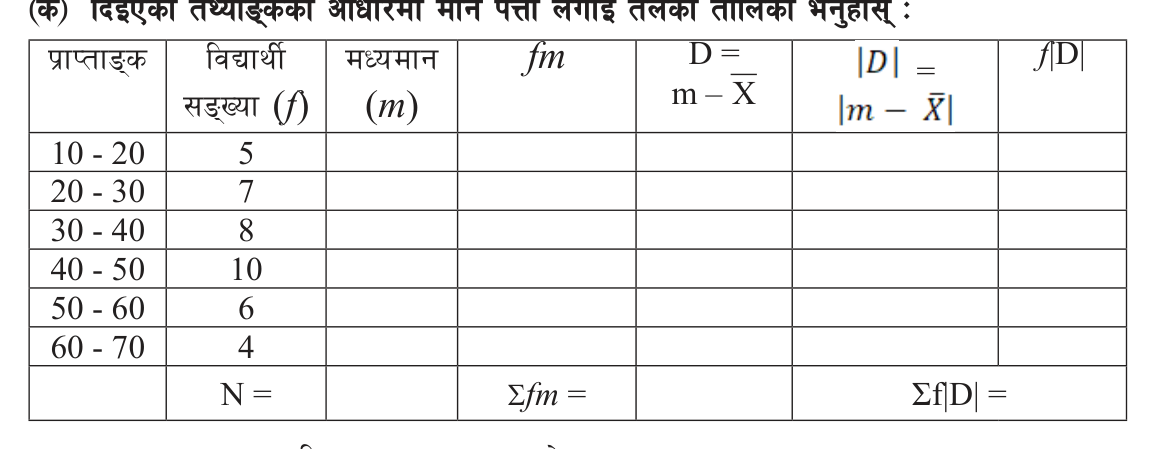
Mean deviation of grouped data is found by building a table one column at a time. For mean deviation from the mean, the columns are:
- Class and frequency f, copied from the data. Their total is N.
- Mid-value m of each class: the lower limit plus the upper limit, divided by 2.
- fm, each frequency times its mid-value. Its total \( \Sigma fm \) gives the mean.
- \( D = m - \bar{X} \), the deviation of each mid-value from the mean.
- \( |D| \), the same deviation with its sign dropped.
- \( f|D| \), each absolute deviation times its frequency. Its total \( \Sigma f|D| \) goes into the formula.
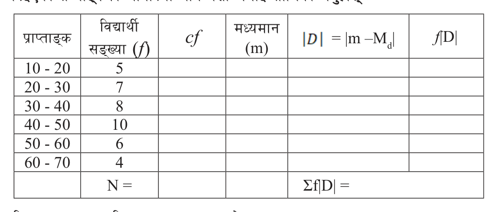
For mean deviation from the median, the fm column is not needed. Instead, a cumulative frequency column cf is added so that the median class can be found, and \( |D| \) is measured from the median.
Worked Example 1: Mean Deviation from the Mean
The weights of 40 students of class 10 in a school lie from 35 kg up to less than 70 kg, as shown in the table. Find the mean deviation from the mean and its coefficient.
| Weight (kg) | Number of students |
| More than 35 | 40 |
| More than 40 | 36 |
| More than 45 | 30 |
| More than 50 | 20 |
| More than 55 | 15 |
| More than 60 | 10 |
| More than 65 | 4 |
This is a cumulative table. 40 students weigh more than 35 kg and 36 weigh more than 40 kg, so the difference, 4 students, weigh from 35 kg up to 40 kg. Each class frequency is one count minus the next. The last figure, 4 students weighing more than 65 kg, is already the frequency of the class 65 - 70.
Never use the figures of a 'more than' or 'less than' table as frequencies. Change them into class frequencies first, and check that the frequencies add up to N.
Step 1: Changing the cumulative figures into class frequencies. For the first class:
\[ f = 40 - 36 = 4 \]
Step 2: Finding the mid-value of each class. For the first class:
\[ m = \frac{35 + 40}{2} = 37.5 \]
Step 3: Multiplying each frequency by its mid-value and adding. For the first class \( 4 \times 37.5 = 150 \), and the total of the fm column is:
\[ \Sigma fm = 2075 \]
Step 4: Dividing by N to find the mean:
\[ \bar{X} = \frac{\Sigma fm}{N} = \frac{2075}{40} = 51.875 \]
Keep the mean exact while you work. Rounding 51.875 to 52 changes every |D| in the next column, and the final answer drifts away from the correct one.
Step 5: Finding how far each mid-value lies from the mean, with the sign dropped. For the first class:
\[ |D| = |37.5 - 51.875| = 14.375 \]
Step 6: Multiplying each absolute deviation by its frequency. For the first class:
\[ f|D| = 4 \times 14.375 = 57.5 \]
Doing the same for every class gives the complete table:
| Weight (kg) | f | m | fm | |D| | f|D| |
| 35 - 40 | 40 - 36 = 4 | 37.5 | 150 | 14.375 | 57.5 |
| 40 - 45 | 36 - 30 = 6 | 42.5 | 255 | 9.375 | 56.25 |
| 45 - 50 | 30 - 20 = 10 | 47.5 | 475 | 4.375 | 43.75 |
| 50 - 55 | 20 - 15 = 5 | 52.5 | 262.5 | 0.625 | 3.125 |
| 55 - 60 | 15 - 10 = 5 | 57.5 | 287.5 | 5.625 | 28.125 |
| 60 - 65 | 10 - 4 = 6 | 62.5 | 375 | 10.625 | 63.75 |
| 65 - 70 | 4 | 67.5 | 270 | 15.625 | 62.5 |
| Total | N = 40 | Σfm = 2075 | Σf|D| = 315 |
Step 7: Adding the f|D| column:
\[ \Sigma f|D| = 315 \]
Step 8: Dividing by N to get the mean deviation from the mean:
\[ \text{MD} = \frac{\Sigma f|D|}{N} = \frac{315}{40} = 7.875 \]
Step 9: Dividing the mean deviation by the mean to get the coefficient:
\[ \text{Coefficient} = \frac{\text{MD}}{\bar{X}} = \frac{7.875}{51.875} = 0.1518 \]
So the mean deviation from the mean is 7.875 kg and its coefficient is 0.1518. On average, a student's weight lies about 7.9 kg away from the mean weight of 51.875 kg.
Worked Example 2: Mean Deviation from the Median
In a test of 50 full marks, 50 students scored as follows: 0 - 10: 4 students, 10 - 20: 11, 20 - 30: 20, 30 - 40: 10, 40 - 50: 5. Find the mean deviation from the median and its coefficient.
Step 1: Adding the frequencies one after another to make the cumulative frequency column. The cf values are 4, 15, 35, 45 and 50, so the total frequency is:
\[ N = 50 \]
Step 2: Finding the position of the median:
\[ \frac{N}{2} = \frac{50}{2} = 25 \]
Step 3: Locating the median class. The first cf that is 25 or more is 35, which belongs to the class 20 - 30. So \( L = 20 \), \( cf = 15 \), \( f = 20 \) and \( i = 10 \). Putting these into the median formula:
\[ M_d = 20 + \frac{25 - 15}{20} \times 10 \]
Step 4: Simplifying, since \( \frac{10}{20} \times 10 = 5 \):
\[ M_d = 20 + 5 = 25 \]
Step 5: Finding each absolute deviation from the median and multiplying by its frequency. For the first class, \( |5 - 25| = 20 \) and:
\[ f|D| = 4 \times 20 = 80 \]
The complete table is:
| Marks | f | cf | m | |D| = |m - 25| | f|D| |
| 0 - 10 | 4 | 4 | 5 | 20 | 80 |
| 10 - 20 | 11 | 15 | 15 | 10 | 110 |
| 20 - 30 | 20 | 35 | 25 | 0 | 0 |
| 30 - 40 | 10 | 45 | 35 | 10 | 100 |
| 40 - 50 | 5 | 50 | 45 | 20 | 100 |
| Total | N = 50 | Σf|D| = 390 |
Step 6: Dividing the total by N to get the mean deviation from the median:
\[ \text{MD} = \frac{\Sigma f|D|}{N} = \frac{390}{50} = 7.8 \]
Step 7: Dividing by the median to get the coefficient:
\[ \text{Coefficient} = \frac{\text{MD}}{M_d} = \frac{7.8}{25} = 0.312 \]
So the mean deviation from the median is 7.8 marks and its coefficient is 0.312. For the same data the mean is \( \frac{1260}{50} = 25.2 \), and the mean deviation from the mean works out to 7.88 marks. The two answers are close but not equal, because the distances are measured from two different centres. Always read the question to see which centre it asks for.
Using the Coefficient to Compare
The mean deviation of the weights in Example 1 is 7.875 kg, and the mean deviation of the marks in Example 2 is 7.8 marks. The two numbers look almost the same, but they cannot be compared directly. One is in kilograms and the other is in marks, and the averages they are spread around are very different: about 52 kg in one case and 25 marks in the other.
The coefficient solves this. Dividing by the average removes the unit and turns the spread into a fraction of the centre. The weights have a coefficient of 0.1518, so their spread is about 15% of their mean. The marks have a coefficient of 0.312, so their spread is about 31% of their median. The marks are therefore spread out much more, relative to their centre, than the weights are.
When two sets of data are compared, the one with the smaller coefficient of mean deviation is more uniform, or more consistent. The one with the larger coefficient is more spread out.
This is how two sections of a class, or two unit tests, can be compared. If section A has a coefficient of 0.18 and section B has 0.27, the marks of section A are closer together, so section A performed more evenly.
What the Size of the Mean Deviation Tells You
- Mean deviation is never negative, because it is an average of absolute values.
- If every item of the data is the same, every |D| is 0, so the mean deviation is 0. For example, if all 30 students in a class score 45 marks, there is no spread at all.
- The larger the mean deviation, the more widely the items are spread around their centre.
- Mean deviation has the same unit as the data: kilograms, marks, rupees. Its coefficient has no unit.
The full lesson is waiting for you
The notes are free to read in full. A free account opens the rest of the practice, and tracks your progress and confidence score for every subject. Presentations and videos need approval from Learn Yeti.