Centre and Spread
Suppose everyone in your class measures their height in centimetres and writes it on the board. The mean, the median and the mode tell you where the middle of those heights lies. They tell you nothing about whether the heights are bunched close together or scattered far apart. Two classes can have exactly the same average height while one has students of almost equal height and the other has some very short and some very tall students.
A measure of central tendency describes the centre of a set of data. A measure of dispersion describes its spread. Neither is enough alone, and a set of data is understood fully only when both are known. Range, quartile deviation, mean deviation and standard deviation are all measures of spread. Quartile deviation is the one that measures spread using only the middle half of the data.
Continuous Series
Imagine the weights of 40 students, recorded to the nearest half kilogram or closer: 35 kg, 39.5 kg, 42 kg, 56.4 kg and so on. Writing each weight in its own row would give a table of 40 lines that nobody could read at a glance. Instead, the whole range of weights is cut into equal pieces called class intervals, and we count how many students fall into each piece. Tally marks make the counting easy: one stroke for each student, with every fifth stroke drawn across the four before it.
Class interval: a group such as 50 - 55 into which values are collected. The smaller number is the lower limit, the larger number is the upper limit, and the difference between them is the width of the class interval.
A class interval written as 55 - 60 means 55 kg or more, but less than 60 kg. So weights of 55, 56, 56.5, 57, 58, 59 and 59.5 kg all belong to the class 55 - 60. A weight of exactly 60 kg does not. It goes into the next class, 60 - 65. Each boundary value belongs to the class that begins with it.
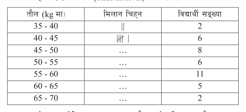
Because the classes join one another without a gap, every possible weight from 35 kg up to 70 kg, whole number or decimal, has exactly one class to go into. Data arranged in this way is called a continuous series.
Continuous series: data that can take decimal values as well as whole-number values, spread over a fixed range, and grouped into class intervals that follow one another without gaps.
The same class is sometimes written with inequality signs. A class shown as \( 20 \le x < 30 \) means that x is 20 or more but less than 30. That is exactly the class 20 - 30.
A value equal to the upper limit of a class is never counted in that class. When you tally a weight of 60 kg, put it in 60 - 65, not in 55 - 60.
Quartiles
Arrange a set of data in order from the smallest value to the largest and imagine cutting it into four equal parts, each holding a quarter of the values. Three cuts are needed, and the values at the three cutting points are called the quartiles.
First quartile or lower quartile \( (Q_1) \): the value that divides the data so that 25% of the values lie below it and 75% lie above it.
Second quartile \( (Q_2) \): the value that divides the data into two halves, 50% below and 50% above. The second quartile is the median.
Third quartile or upper quartile \( (Q_3) \): the value that divides the data so that 75% of the values lie below it and 25% lie above it.
So the lowest quarter of the data sits below \( Q_1 \), the highest quarter sits above \( Q_3 \), and exactly the middle 50% of the data lies between \( Q_1 \) and \( Q_3 \).
Interquartile Range and Quartile Deviation
Interquartile range: the difference between the third (upper) quartile and the first (lower) quartile.
\[ \text{Interquartile range} = Q_3 - Q_1 \]
Quartile deviation (Q.D.), also called the semi-interquartile range: half of the difference between the upper quartile and the lower quartile.
\[ \text{Q.D.} = \frac{Q_3 - Q_1}{2} \]
Quartile deviation leaves out the lowest 25% and the highest 25% of the values completely. This makes it useful when a set of data has one or two unusual values at its ends. Think of the monthly incomes of the families in a village where one family is very rich. The range of incomes becomes huge because of that one family. The quartile deviation hardly changes, because the richest family lies in the top quarter, which is left out.
A small quartile deviation means the middle half of the data is packed closely together. A large quartile deviation means the middle half is widely spread. The quartile deviation always has the same unit as the data: if the data are weights in kg, the Q.D. is in kg too.
Quartile deviation measures how spread out the middle half of the data is. It uses only \( Q_1 \) and \( Q_3 \), so extreme values at either end do not affect it.
Coefficient of Quartile Deviation
The quartile deviation alone cannot compare two series measured in different units, or series whose values are of very different sizes. A spread of 5 kg in the weights of students and a spread of 5 rupees in their pocket money cannot be compared directly. For such comparisons we divide the difference of the quartiles by their sum. The units cancel and a pure number is left.
Coefficient of quartile deviation: the ratio of the difference between the upper and lower quartiles to their sum. It has no unit.
In symbols, the coefficient of quartile deviation is:
\[ \frac{Q_3 - Q_1}{Q_3 + Q_1} \]
When two series are compared, the one with the smaller coefficient has its middle half more tightly grouped, so it is the more consistent of the two.
Finding the First and Third Quartiles
In a continuous series the individual values are no longer visible. We know only how many values lie in each class. So a quartile is found in two stages. First we find the class in which the quartile lies. Then we estimate how far into that class it falls, assuming the values inside the class are spread evenly across it. The method is always the same:
- Write the class intervals and their frequencies (f) in a table.
- Add a cumulative frequency (cf) column by adding the frequencies one after another. The last cumulative frequency is the total number of values, N.
- Find the position of the first quartile as the \( \frac{N}{4} \)th item, and the position of the third quartile as the \( \frac{3N}{4} \)th item.
- Look down the cf column for the first cumulative frequency that is equal to or greater than that position. The class in that row is the quartile class.
- Read off l, f, cf and i for the quartile class and put them into the formula.
The formula for the first quartile is:
\[ Q_1 = l + \frac{\frac{N}{4} - cf}{f} \times i \]
The formula for the third quartile is the same, with \( \frac{3N}{4} \) in place of \( \frac{N}{4} \):
\[ Q_3 = l + \frac{\frac{3N}{4} - cf}{f} \times i \]
The letters in both formulas mean:
- l is the lower limit of the quartile class.
- f is the frequency of the quartile class.
- cf is the cumulative frequency of the class just before the quartile class.
- i is the width of the class interval, the upper limit minus the lower limit.
- N is the total frequency.
The fraction in the middle of the formula says how far into the quartile class we must go. The top of the fraction counts how many more values are needed after the earlier classes, and the bottom is how many values the quartile class holds.
In the formula, cf is the cumulative frequency of the class BEFORE the quartile class, not of the quartile class itself. If you use the quartile class's own cf, the top of the fraction usually turns negative and the quartile lands below its own class.
Worked Example 1: Daily Wages of Workers
The daily wages of 350 workers, in hundreds of rupees, are given below. Find the quartile deviation and its coefficient.
| Wages (hundreds of rupees) | Number of workers |
| 6 - 8 | 60 |
| 8 - 10 | 75 |
| 10 - 12 | 85 |
| 12 - 14 | 70 |
| 14 - 16 | 50 |
| 16 - 18 | 10 |
Step 1: Building the cumulative frequency column by adding each frequency to the total so far. For example, the second cf is 60 + 75 = 135:
| Wages | f | cf |
| 6 - 8 | 60 | 60 |
| 8 - 10 | 75 | 135 |
| 10 - 12 | 85 | 220 |
| 12 - 14 | 70 | 290 |
| 14 - 16 | 50 | 340 |
| 16 - 18 | 10 | 350 |
| N = 350 |
Step 2: Finding the position of the first quartile:
\[ \frac{N}{4} = \frac{350}{4} = 87.5 \]
Step 3: Locating the class of \( Q_1 \). The first cf equal to or greater than 87.5 is 135, so the 87.5th item lies in the class 8 - 10. The class before it has cf 60. Reading off the values:
\[ l = 8,\; f = 75,\; cf = 60,\; i = 10 - 8 = 2 \]
Step 4: Substituting these values into the formula for \( Q_1 \):
\[ Q_1 = 8 + \frac{87.5 - 60}{75} \times 2 \]
Step 5: Simplifying. Since \( \frac{27.5}{75} \times 2 = 0.73 \) to two decimal places:
\[ Q_1 = 8 + 0.73 = 8.73 \]
Step 6: Finding the position of the third quartile:
\[ \frac{3N}{4} = \frac{3 \times 350}{4} = 262.5 \]
Step 7: Locating the class of \( Q_3 \). The first cf equal to or greater than 262.5 is 290, so the class is 12 - 14. The class before it has cf 220. Reading off the values:
\[ l = 12,\; f = 70,\; cf = 220,\; i = 2 \]
Step 8: Substituting into the formula for \( Q_3 \):
\[ Q_3 = 12 + \frac{262.5 - 220}{70} \times 2 \]
Step 9: Simplifying. Since \( \frac{42.5}{70} \times 2 = 1.21 \) to two decimal places:
\[ Q_3 = 12 + 1.21 = 13.21 \]
Step 10: Halving the difference of the quartiles to get the quartile deviation:
\[ \text{Q.D.} = \frac{13.21 - 8.73}{2} = \frac{4.48}{2} = 2.24 \]
Step 11: Dividing the difference of the quartiles by their sum to get the coefficient:
\[ \frac{13.21 - 8.73}{13.21 + 8.73} = \frac{4.48}{21.94} = 0.20 \]
So the quartile deviation is 2.24 hundred rupees, which is Rs. 224, and the coefficient of quartile deviation is 0.20. The middle half of the workers earn wages that are spread about Rs. 224 on either side of the centre of that middle half.
Worked Example 2: A Less Than Table
Sometimes data are given as a "less than" table. Each figure then counts everything below a value, so it is already a cumulative frequency. The frequency of each class must be recovered by subtraction before the formula can be used. The table below shows how many hours a day 30 workers work. Find the quartile deviation and its coefficient.
| Working time (hours) | Number of workers |
| Less than 2 | 5 |
| Less than 4 | 7 |
| Less than 6 | 8 |
| Less than 8 | 15 |
| Less than 10 | 25 |
| Less than 12 | 30 |
Step 1: Finding the frequency of each class by subtracting the figure before it. For the class 2 - 4, the workers who work less than 4 hours but not less than 2 hours number:
\[ f = 7 - 5 = 2 \]
Step 2: Doing the same for every class. The "less than" figures become the cf column:
| Hours | f | cf |
| 0 - 2 | 5 | 5 |
| 2 - 4 | 7 - 5 = 2 | 7 |
| 4 - 6 | 8 - 7 = 1 | 8 |
| 6 - 8 | 15 - 8 = 7 | 15 |
| 8 - 10 | 25 - 15 = 10 | 25 |
| 10 - 12 | 30 - 25 = 5 | 30 |
| N = 30 |
Step 3: Finding the position of the first quartile:
\[ \frac{N}{4} = \frac{30}{4} = 7.5 \]
Step 4: Locating the class of \( Q_1 \). The cf values run 5, 7, 8, and the first one equal to or greater than 7.5 is 8, so the class is 4 - 6. The class before it has cf 7:
\[ l = 4,\; f = 1,\; cf = 7,\; i = 2 \]
Step 5: Substituting into the formula for \( Q_1 \):
\[ Q_1 = 4 + \frac{7.5 - 7}{1} \times 2 \]
\[ Q_1 = 4 + 1 = 5 \]
Step 6: Finding the position of the third quartile:
\[ \frac{3N}{4} = \frac{3 \times 30}{4} = 22.5 \]
Step 7: Locating the class of \( Q_3 \). The first cf equal to or greater than 22.5 is 25, so the class is 8 - 10. The class before it has cf 15:
\[ l = 8,\; f = 10,\; cf = 15,\; i = 2 \]
Step 8: Substituting into the formula for \( Q_3 \):
\[ Q_3 = 8 + \frac{22.5 - 15}{10} \times 2 \]
\[ Q_3 = 8 + 1.5 = 9.5 \]
Step 9: Halving the difference of the quartiles:
\[ \text{Q.D.} = \frac{9.5 - 5}{2} = \frac{4.5}{2} = 2.25 \]
Step 10: Dividing the difference of the quartiles by their sum:
\[ \frac{9.5 - 5}{9.5 + 5} = \frac{4.5}{14.5} = 0.31 \]
So the quartile deviation is 2.25 hours and the coefficient of quartile deviation is 0.31.
Worked Example 3: A More Than Table
A "more than" table counts everything above a value, so its figures fall as you move down the table. Again, each class frequency is found by subtraction, this time taking the NEXT figure away from the current one. The marks of 60 students in a test out of 50 are given below. Find the quartile deviation and its coefficient.
| Marks | Number of students |
| More than 0 | 60 |
| More than 10 | 52 |
| More than 20 | 36 |
| More than 30 | 16 |
| More than 40 | 4 |
Step 1: Finding the frequency of the class 0 - 10. Of the 60 students who scored more than 0, there are 52 who scored more than 10, so the rest scored from 0 up to 10:
\[ f = 60 - 52 = 8 \]
Step 2: Doing the same for every class and then adding a cf column from the top. The last class, 40 - 50, keeps its figure of 4 because nobody can score above 50:
| Marks | f | cf |
| 0 - 10 | 60 - 52 = 8 | 8 |
| 10 - 20 | 52 - 36 = 16 | 24 |
| 20 - 30 | 36 - 16 = 20 | 44 |
| 30 - 40 | 16 - 4 = 12 | 56 |
| 40 - 50 | 4 | 60 |
| N = 60 |
Step 3: Finding the position of the first quartile:
\[ \frac{N}{4} = \frac{60}{4} = 15 \]
Step 4: Locating the class of \( Q_1 \). The first cf equal to or greater than 15 is 24, so the class is 10 - 20. The class before it has cf 8:
\[ l = 10,\; f = 16,\; cf = 8,\; i = 10 \]
Step 5: Substituting into the formula for \( Q_1 \):
\[ Q_1 = 10 + \frac{15 - 8}{16} \times 10 \]
\[ Q_1 = 10 + 4.375 = 14.375 \]
Step 6: Finding the position of the third quartile:
\[ \frac{3N}{4} = \frac{3 \times 60}{4} = 45 \]
Step 7: Locating the class of \( Q_3 \). The cf 44 is just short of 45, so the first cf equal to or greater than 45 is 56, and the class is 30 - 40. The class before it has cf 44:
\[ l = 30,\; f = 12,\; cf = 44,\; i = 10 \]
Step 8: Substituting into the formula for \( Q_3 \):
\[ Q_3 = 30 + \frac{45 - 44}{12} \times 10 \]
\[ Q_3 = 30 + 0.83 = 30.83 \]
Step 9: Halving the difference of the quartiles:
\[ \text{Q.D.} = \frac{30.83 - 14.375}{2} \]
\[ \text{Q.D.} = \frac{16.455}{2} = 8.23 \]
Step 10: Dividing the difference of the quartiles by their sum:
\[ \frac{30.83 - 14.375}{30.83 + 14.375} \]
\[ = \frac{16.455}{45.205} = 0.36 \]
So the quartile deviation is 8.23 marks and the coefficient of quartile deviation is 0.36.
In a "more than" table the figures are not cumulative frequencies in the usual order. Do not copy them straight into the cf column. Find each class frequency first, then build the cf column again from the top.
Can the Coefficient Be More Than 1?
Marks, weights, wages and hours are never negative, so for such data \( Q_1 \) is 0 or more. Taking a number of 0 or more away from \( Q_3 \) can never give more than adding it to \( Q_3 \). So \( Q_3 - Q_1 \) is never bigger than \( Q_3 + Q_1 \), and the coefficient of quartile deviation always lies between 0 and 1.
The coefficient is 0 when \( Q_1 = Q_3 \), which happens only if the whole middle half of the data has the same value. It could reach 1 only if \( Q_1 \) were 0. The three worked examples above give 0.20, 0.31 and 0.36, all comfortably inside that range.
If your coefficient of quartile deviation comes out greater than 1, or negative, there is a mistake. The usual causes are swapping \( Q_1 \) and \( Q_3 \), or dividing by the difference instead of the sum.
The full lesson is waiting for you
The notes are free to read in full. A free account opens the rest of the practice, and tracks your progress and confidence score for every subject. Presentations and videos need approval from Learn Yeti.