Same Average, Different Spread
Asha and Bikash each sat five class tests, marked out of 100. Here are their marks.
| Student | Test 1 | Test 2 | Test 3 | Test 4 | Test 5 | Total | Mean |
| Asha | 62 | 65 | 64 | 66 | 63 | 320 | 64 |
| Bikash | 44 | 84 | 54 | 74 | 64 | 320 | 64 |
Both students have a mean of 64. If we look only at the average, they seem equally good. The marks tell a different story. Asha never drops below 62 and never rises above 66, so her marks sit tightly around 64. Bikash swings from 44 all the way up to 84. Some of his tests go very well and others go badly.
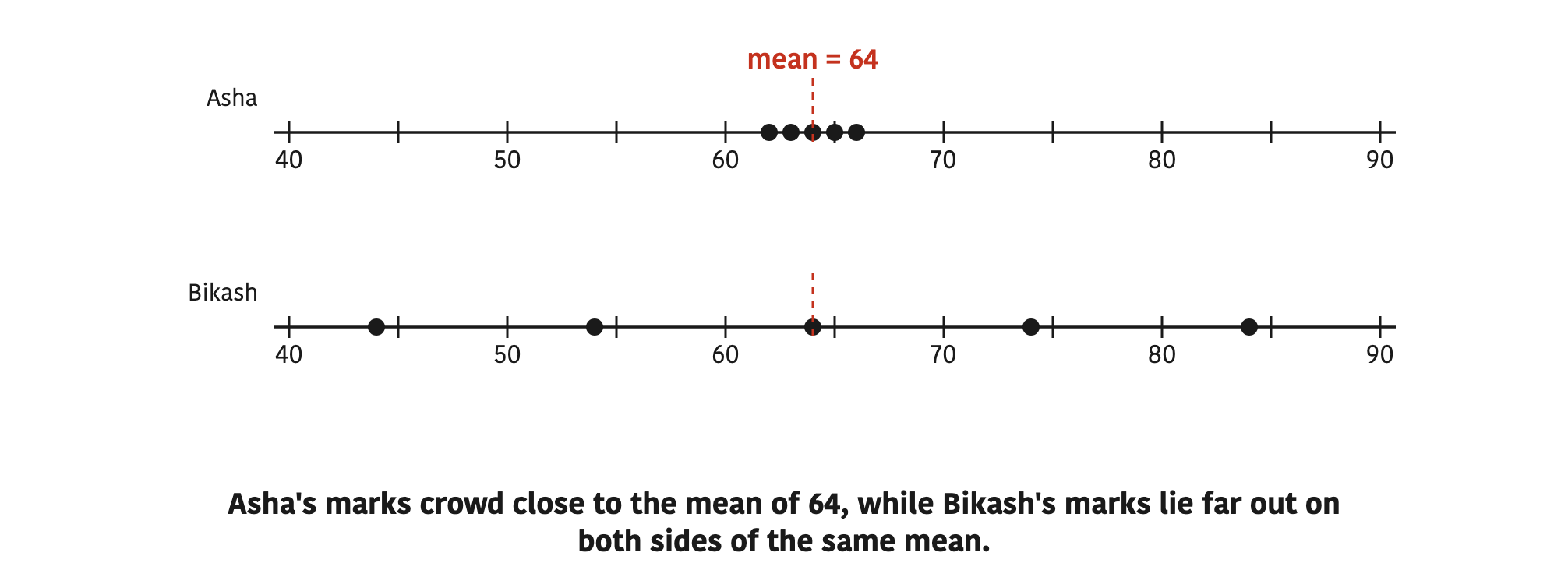
So a mean on its own cannot tell us whether a set of values is steady or up and down. We also need a number that says how widely the values are scattered around the mean. Such a number is a measure of dispersion. You already know three of them: range, quartile deviation and mean deviation. The fourth, and the most important, is standard deviation.
11.4 Standard Deviation
Standard deviation is the measure of dispersion that tells how far or how near the values of a data set are scattered from their mean. It is written with the small Greek letter \( \sigma \), read as small sigma.
Of all the measures of dispersion (range, quartile deviation, mean deviation and standard deviation), standard deviation is the one used most often, and it is accepted as the most standard measure of spread.
Variance is the square of the standard deviation. It is written \( \sigma^2 \).
The idea behind \( \sigma \) is simple. Find how far each value is from the mean. Square those distances, so that no negative sign can cancel a positive one. Take the average of the squares. Finally take the square root, which brings the answer back to the unit of the data. For n separate values x with mean \( \bar{X} \), this is written as:
\[ \sigma = \sqrt{\frac{\sum (x - \bar{X})^2}{n}} \]
Here \( \sum \) means add them all up, \( x - \bar{X} \) is the deviation of one value from the mean, and n is the number of values. The quantity under the square root sign is the variance:
\[ \sigma^2 = \frac{\sum (x - \bar{X})^2}{n} \]
For data arranged in a frequency table, exactly the same idea is applied to the mid values of the classes and their frequencies.
Worked Example 1: Standard Deviation of Two Students' Marks
Find the variance and the standard deviation of Asha's marks: 62, 65, 64, 66, 63.
Step 1: Finding the mean by adding the five marks and dividing by 5:
\[ \bar{X} = \frac{62 + 65 + 64 + 66 + 63}{5} = \frac{320}{5} = 64 \]
Step 2: Subtracting the mean from each mark and squaring each deviation. A table keeps this work tidy:
| \( x \) | \( x - \bar{X} \) | \( (x - \bar{X})^2 \) |
| 62 | -2 | 4 |
| 65 | 1 | 1 |
| 64 | 0 | 0 |
| 66 | 2 | 4 |
| 63 | -1 | 1 |
| Total | 0 | 10 |
Step 3: Dividing the sum of the squares by the number of marks gives the variance:
\[ \sigma^2 = \frac{10}{5} = 2 \]
Step 4: Taking the square root of the variance gives the standard deviation:
\[ \sigma = \sqrt{2} \approx 1.41 \]
The same four steps work for Bikash's marks 44, 84, 54, 74 and 64. His mean is 64 again. His deviations are -20, 20, -10, 10 and 0, and their squares are 400, 400, 100, 100 and 0. Adding the squares and dividing by 5 gives his variance:
\[ \sigma^2 = \frac{1000}{5} = 200 \]
Taking the square root gives his standard deviation:
\[ \sigma = \sqrt{200} \approx 14.14 \]
The deviations \( x - \bar{X} \) always add up to 0, as the Total row shows. That is exactly why they are squared before they are added. Adding the plain deviations will always give 0 and tells you nothing about the spread.
Reading the Value of Standard Deviation
Asha's standard deviation is about 1.41 marks and Bikash's is about 14.14 marks, even though both means are 64. The standard deviation is measured in the same unit as the data, so here it is in marks.
When two sets of data have the same mean, the one with the smaller standard deviation is more uniform, more consistent and more stable. The one with the larger standard deviation is more scattered and more variable.
So Asha is the more consistent student. On any test you can expect her to score close to 64. With Bikash you cannot be sure: he might score in the 80s or in the 40s. A standard deviation of 0 would mean every value is exactly equal to the mean, with no spread at all.
Why Standard Deviation Is the Best Measure of Dispersion
Each of the other measures of dispersion has a weakness. Standard deviation avoids them, and that is why it is taken as the most suitable measure:
- It uses every value in the data. Range uses only the largest and the smallest value, and quartile deviation uses only the two quartiles.
- It measures every deviation from the mean, which is the natural centre of the data.
- It squares the deviations, so the negative signs disappear by proper algebra. Mean deviation simply ignores the signs, which makes it hard to use in further calculation.
- It is in the same unit as the data, so its value can be read directly.
- Many further results in statistics, including the coefficient of variation, are built on it.
11.4.1 Uses of Standard Deviation
Standard deviation is one of the most important measures of dispersion, and it is used in many fields. Wherever people want to know not only the average but also how steady something is, standard deviation is the tool they use.
- Education: to compare how equal or unequal students' exam results are. A class with a small standard deviation has marks close together, while a class with a large one has a wide gap between strong and weak students.
- Weather forecasting: to measure how much temperature or rainfall rises and falls around its average. A town whose daily temperature has a small standard deviation has a steady climate.
- Share market: to find how much risk there is in a stock or an investment. A share whose price has a large standard deviation can jump up or crash down quickly, so it is riskier.
- Quality control: to make sure the goods a factory produces are all of the same quality. If every packet of noodles should weigh 70 g, a small standard deviation in the weights shows the machine is filling them evenly.
11.4.2 Coefficient of Standard Deviation
The coefficient of standard deviation is the value obtained by dividing the standard deviation by the mean.
\[ \text{Coefficient of S.D.} = \frac{\sigma}{\bar{X}} \]
Why do we need it? A standard deviation carries the unit of its data. Heights in centimetres give a standard deviation in centimetres, and weights in kilograms give one in kilograms. Nobody can say whether 6 cm is more spread out than 5.4 kg, because they are different kinds of quantity. Dividing by the mean cancels the unit and leaves a pure number, so data in different units can be compared. It also takes care of different means: a spread of 5 around a mean of 10 is huge, but a spread of 5 around a mean of 1000 is tiny.
The smaller the coefficient of standard deviation, the more uniformity or stability the data have. The larger it is, the less uniform and less stable the data are, and the more variety they show.
Worked Example 2: Comparing Heights and Weights
In a class, the mean height of the students is 150 cm with a standard deviation of 6 cm. Their mean weight is 45 kg with a standard deviation of 5.4 kg. Which vary more, the heights or the weights?
Step 1: Dividing the standard deviation of the heights by their mean:
\[ \frac{\sigma}{\bar{X}} = \frac{6}{150} = 0.04 \]
Step 2: Dividing the standard deviation of the weights by their mean:
\[ \frac{\sigma}{\bar{X}} = \frac{5.4}{45} = 0.12 \]
Step 3: Comparing the two coefficients. Since 0.12 is greater than 0.04, the weights vary more. The heights of these students are more uniform than their weights. The plain standard deviations, 6 and 5.4, could never have answered this question, because one is in centimetres and the other in kilograms.
11.5 Coefficient of Variation
The coefficient of variation is the coefficient of standard deviation expressed as a percentage. It is written C.V.
\[ \text{C.V.} = \frac{\sigma}{\bar{X}} \times 100\% \]
The coefficient of standard deviation usually comes out as a decimal between 0 and 1, such as 0.04 or 0.12. Decimals like these are awkward to compare at a glance, so they are changed into percentages: 4% and 12%. The C.V. is read in exactly the same way as the coefficient of standard deviation.
A smaller C.V. means more uniform, more consistent and more stable data. A larger C.V. means less uniform, less stable data with more variety.
For Asha, whose mean is 64 and standard deviation about 1.41:
\[ \text{C.V.} = \frac{1.41}{64} \times 100\% \approx 2.20\% \]
For Bikash, whose mean is 64 and standard deviation about 14.14:
\[ \text{C.V.} = \frac{14.14}{64} \times 100\% \approx 22.09\% \]
Bikash's C.V. is about ten times Asha's, so his marks are far less consistent than hers.
Worked Example 3: Which Batsman Is More Consistent?
Over one season, batsman P scored a mean of 48 runs per innings with a standard deviation of 12 runs. Batsman Q scored a mean of 40 runs per innings with a standard deviation of 6 runs. Who is the better run scorer, and who is more consistent?
Step 1: Finding the C.V. of batsman P:
\[ \text{C.V.} = \frac{12}{48} \times 100\% = 25\% \]
Step 2: Finding the C.V. of batsman Q:
\[ \text{C.V.} = \frac{6}{40} \times 100\% = 15\% \]
Step 3: Reading the results. P has the higher mean, so P is the better run scorer. Q has the smaller C.V., 15% against 25%, so Q is the more consistent batsman. A captain who needs a steady score every match would choose Q. A captain hoping for one big innings might take a chance on P.
A smaller C.V. does not mean a smaller average. It only means the values stay closer to their own average. Answer who scores more by looking at the mean, and who is more consistent by looking at the C.V.
Worked Example 4: Working Back from the Coefficient of Variation
The C.V. of a set of data is 20% and its mean is 60. Find the standard deviation and the variance.
Step 1: Putting the known values into the formula for C.V.:
\[ 20 = \frac{\sigma}{60} \times 100 \]
Step 2: Multiplying both sides by 60 and dividing by 100 to make \( \sigma \) the subject:
\[ \sigma = \frac{20 \times 60}{100} = 12 \]
Step 3: Squaring the standard deviation to get the variance:
\[ \sigma^2 = 12^2 = 144 \]
The formula works in every direction: if you know any two of \( \sigma \), \( \bar{X} \) and C.V., you can find the third. For example, when the variance is 25 and the mean is 50, first \( \sigma = \sqrt{25} = 5 \), and then:
\[ \text{C.V.} = \frac{5}{50} \times 100\% = 10\% \]
When the variance is given, take its square root before using the formula. Putting the variance in place of \( \sigma \) gives a C.V. that is far too large: here it would give 50% instead of 10%.
The Formulas at a Glance
| Quantity | Symbol or formula | How to read it |
| Standard deviation | \( \sigma \) | Spread in the unit of the data; smaller is steadier |
| Variance | \( \sigma^2 \) | The square of the standard deviation |
| Coefficient of S.D. | \( \frac{\sigma}{\bar{X}} \) | No unit; smaller is more uniform |
| Coefficient of variation | \( \frac{\sigma}{\bar{X}} \times 100\% \) | A percentage; smaller is more consistent |
The full lesson is waiting for you
The notes are free to read in full. A free account opens the rest of the practice, and tracks your progress and confidence score for every subject. Presentations and videos need approval from Learn Yeti.