Averages of a List of Marks
Statistics starts with a list of numbers. Twenty-seven students of class 10 scored these marks in mathematics in their second terminal examination:
25, 15, 30, 22, 27, 12, 25, 30, 22, 24, 15, 23, 19, 27, 28, 17, 19, 22, 25, 15, 14, 13, 28, 26, 18, 20, 22
The average of these marks is called the mean. It is the total of all the marks divided by the number of students. The 27 marks add up to 583, so:
\[ \overline{X} = \frac{583}{27} \approx 21.59 \]
Arranged from lowest to highest, the marks are 12, 13, 14, 15, 15, 15, 17, 18, 19, 19, 20, 22, 22, 22, 22, 23, 24, 25, 25, 25, 26, 27, 27, 28, 28, 30, 30. The first eleven of them, up to 20, are below the mean. So 11 students scored less than the average and the other 16 scored more. The same ordered list gives the other central values you already know:
- Median: the middle mark, the 14th, which is 22.
- First quartile: the 7th mark, which is 17.
- Third quartile: the 21st mark, which is 26.
- Mode: the mark scored by the most students. Four students scored 22, more than any other mark, so the mode is 22.
Arithmetic mean: the sum of all the observations divided by the number of observations. It is written \( \overline{X} \) and read as 'X bar'.
Adding 27 marks by hand is easy. When there are hundreds of observations, or the same values come again and again, we need a quicker and tidier way to find the mean.
Mean of a Discrete Series
When values repeat, we do not write every one of them. We write each different value \( x \) once, together with its frequency \( f \), the number of times it occurs. To find the mean, each value is multiplied by its frequency, the products are added, and the total is divided by the sum of the frequencies:
\[ \overline{X} = \frac{f_1x_1 + f_2x_2 + \dots + f_nx_n}{f_1 + f_2 + \dots + f_n} \]
Writing \( \sum \) (sigma) for 'the sum of', this becomes short:
\[ \overline{X} = \frac{\sum fx}{\sum f} = \frac{\sum fx}{n} \]
Here \( n = \sum f \) is the total number of observations.
Frequency: the number of times a value, or a class of values, occurs in the data. It is written f.
Discrete series: data written as separate values, each with its frequency, such as 3 members in 4 houses, 4 members in 7 houses.
A survey of 20 houses in a tole counted the family members in each house:
| Family members (x) | Houses (f) | fx |
| 3 | 4 | 12 |
| 4 | 7 | 28 |
| 5 | 5 | 25 |
| 6 | 3 | 18 |
| 7 | 1 | 7 |
| Total | Σf = 20 | Σfx = 90 |
Step 1: Multiplying each value by its frequency gives the fx column. Adding that column:
\[ \sum fx = 12 + 28 + 25 + 18 + 7 = 90 \]
Step 2: Adding the frequencies to get the number of houses:
\[ \sum f = 4 + 7 + 5 + 3 + 1 = 20 \]
Step 3: Dividing the total number of members by the number of houses:
\[ \overline{X} = \frac{90}{20} = 4.5 \]
So a house in this tole has 4.5 members on average. A mean does not have to be one of the values in the data, and it does not have to be a whole number.
Grouping Raw Data into a Continuous Series
Data just as it was collected, before any arranging, is called raw data. When raw data is long and spread over many different values, a table that lists every value on its own row becomes very large. The way out is to collect the values into groups.

For example, 40 students of class 9 scored these marks in mathematics:
25, 10, 31, 22, 37, 42, 45, 37, 32, 34, 45, 40, 29, 27, 28, 17, 19, 22, 25, 33, 15, 14, 13, 28, 36, 38, 41, 42, 39, 25, 24, 31, 21, 22, 25, 26, 35, 36, 39, 49
The lowest mark is 10 and the highest is 49. Taking a class interval of 10, every mark fits into one of four classes: 10-20, 20-30, 30-40 and 40-50. The table is built like this:
- Find the lowest and the highest value in the data.
- Choose a class interval and write the classes one below another, starting from a class that contains the lowest value.
- Read the data one value at a time and draw a tally bar against the class it belongs to. Every fifth bar is drawn across the four before it, so the bars can be counted in fives.
- Count the tally bars of each class and write the number as its frequency.
- Add the frequencies and check that the total equals the number of values in the data.
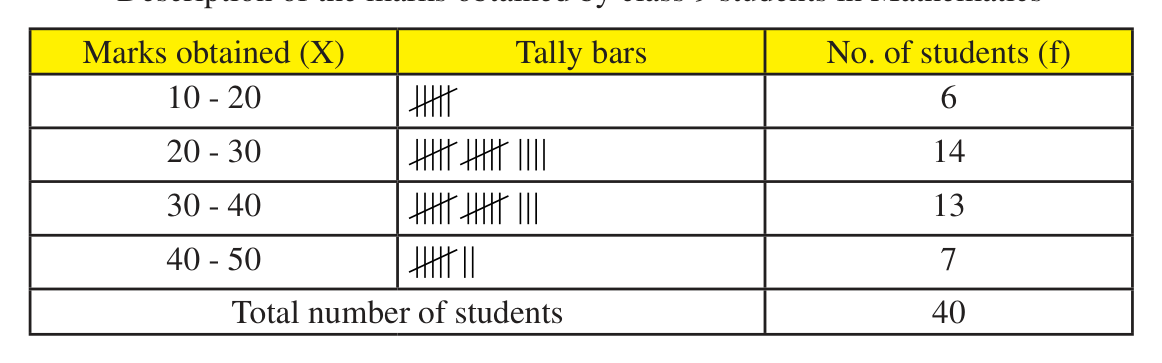
The number of students in each class is the frequency of that class. Adding the frequencies, \( 6 + 14 + 13 + 7 = 40 \), shows that no mark has been missed and none has been counted twice.
In classes written 10-20, 20-30, 30-40, a value equal to an upper limit is not counted in that class. A mark of exactly 20 goes into 20-30, and a mark of exactly 40 goes into 40-50. Putting it in both classes makes the total bigger than the number of students.
Class interval: a group such as 10-20 into which the data is sorted. Here 10 is the lower limit, 20 is the upper limit, and their difference, 10, is the length of the class interval, written h.
Continuous series: data arranged in class intervals that follow one another without a gap, such as 10-20, 20-30, 30-40, with the frequency of each class.
Frequency table: a table that shows each value or class together with its frequency.
Mid-value of a Class Interval
Once the marks are grouped, we no longer know each student's exact mark. We only know, for example, that 6 students scored from 10 up to 20. To calculate with a class, we let the number exactly in its middle stand for the whole class. This number is the mid-value, written m:
\[ m = \frac{\text{lower limit} + \text{upper limit}}{2} \]
For the class 10-20, \( m = \frac{10 + 20}{2} = 15 \). In the same way the classes 20-30, 30-40 and 40-50 have mid-values 25, 35 and 45. A mid-value can be a decimal: the class 140-145 has \( m = \frac{140 + 145}{2} = 142.5 \).
Mid-value: the number halfway between the lower and upper limits of a class interval. It stands for every value in that class when the mean is calculated.
When every class has its mid-value, the continuous series is handled just like a discrete series, with m taking the place of x.
Direct Method
In the direct method, each frequency is multiplied by its mid-value, these products are added, and the total is divided by the total frequency N:
\[ \overline{X} = \frac{\sum fm}{N} \]
Here \( N = \sum f \), the total number of observations.
Direct method: finding the mean of a continuous series straight from the products of frequency and mid-value, using \( \overline{X} = \frac{\sum fm}{N} \).
Here is the working table for the 40 marks of class 9 students:
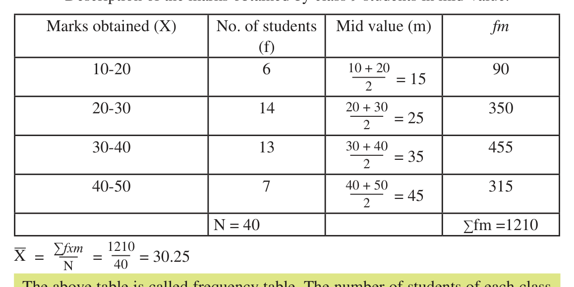
Step 1: Finding the mid-value of the first class:
\[ m = \frac{10 + 20}{2} = 15 \]
Step 2: The other mid-values are 25, 35 and 45. Multiplying each frequency by its mid-value gives 90, 350, 455 and 315. Adding these products:
\[ \sum fm = 90 + 350 + 455 + 315 = 1210 \]
Step 3: Adding the frequencies:
\[ N = 6 + 14 + 13 + 7 = 40 \]
Step 4: Dividing the sum of the products by N:
\[ \overline{X} = \frac{1210}{40} = 30.25 \]
The mean mark of the 40 students is 30.25. This is the mean of the grouped data, because each class was represented by its mid-value. The 40 raw marks actually add up to 1199, which gives 29.975. The two are very close, and that is why grouping is a fair way to handle a long list.
Assumed Mean Method
Multiplying large mid-values by large frequencies can be slow. The assumed mean method, also called the short-cut method, keeps the numbers small. We take any convenient number as the assumed mean A, usually a mid-value near the middle of the table. Then, for each class, we find how far its mid-value is from A:
\[ d = m - A \]
The mean is then the assumed mean corrected by the average of these deviations:
\[ \overline{X} = A + \frac{\sum fd}{N} \]
Assumed mean: any convenient number, usually one of the mid-values, taken as a starting point so that the working uses smaller numbers. It is written A.
Deviation: the difference between a mid-value and the assumed mean, \( d = m - A \). It is negative when the mid-value is smaller than A.
Here are the same 40 marks, worked with A = 25:
| Marks (X) | f | m | d = m - 25 | fd |
| 10-20 | 6 | 15 | -10 | -60 |
| 20-30 | 14 | 25 | 0 | 0 |
| 30-40 | 13 | 35 | 10 | 130 |
| 40-50 | 7 | 45 | 20 | 140 |
| Total | N = 40 | Σfd = 210 |
Step 1: Taking the assumed mean as 25 and finding the deviation of the first mid-value:
\[ d = 15 - 25 = -10 \]
Step 2: The other deviations are 0, 10 and 20. Multiplying each deviation by its frequency gives -60, 0, 130 and 140. Adding them:
\[ \sum fd = -60 + 0 + 130 + 140 = 210 \]
Step 3: Putting A, Σfd and N into the formula:
\[ \overline{X} = 25 + \frac{210}{40} \]
Step 4: Dividing first, then adding:
\[ \overline{X} = 25 + 5.25 = 30.25 \]
Both methods give 30.25. The assumed mean changes the working, never the answer. With \( A = 35 \) the deviations would be -20, -10, 0 and 10, so \( \sum fd = -190 \) and \( \overline{X} = 35 - \frac{190}{40} = 35 - 4.75 = 30.25 \) once again.
Keep the sign of every deviation. Mid-values smaller than A give a negative d and a negative fd. When \( \sum fd \) is negative, the fraction is taken away from A, so the mean is less than A.
Using the Formulas When Totals Are Given
Sometimes the table has already been worked and only its totals are given. The formula is then used straight away. Find the mean when \( \sum fm = 2700 \) and \( N = 50 \).
Step 1: Writing the formula of the direct method:
\[ \overline{X} = \frac{\sum fm}{N} \]
Step 2: Putting in the totals and dividing:
\[ \overline{X} = \frac{2700}{50} = 54 \]
Now find the mean when the assumed mean \( A = 40 \), \( \sum fd = 20 \) and \( N = 10 \).
Step 1: Putting the values into the assumed mean formula:
\[ \overline{X} = 40 + \frac{20}{10} \]
Step 2: Dividing, then adding:
\[ \overline{X} = 40 + 2 = 42 \]
A formula can also be turned round to find a missing total. If \( \overline{X} = 36 \) and \( N = 25 \), multiplying both sides of \( \overline{X} = \frac{\sum fm}{N} \) by N gives:
\[ \sum fm = \overline{X} \times N = 36 \times 25 = 900 \]
Mean Weight of 88 Students by Both Methods
The weights of 88 students of Ganesh Secondary School are grouped in this table. Find their mean weight.
| Weight (kg) | 10-20 | 20-30 | 30-40 | 40-50 | 50-60 |
| Students | 18 | 27 | 20 | 17 | 6 |
Direct method. The working table is:
| Weight (kg) (X) | f | m | fm |
| 10-20 | 18 | 15 | 270 |
| 20-30 | 27 | 25 | 675 |
| 30-40 | 20 | 35 | 700 |
| 40-50 | 17 | 45 | 765 |
| 50-60 | 6 | 55 | 330 |
| Total | N = 88 | Σfm = 2740 |
Step 1: Adding the fm column:
\[ \sum fm = 270 + 675 + 700 + 765 + 330 = 2740 \]
Step 2: Dividing by the number of students:
\[ \overline{X} = \frac{2740}{88} \approx 31.14 \]
Assumed mean method, taking A = 35, the mid-value of the middle class:
| Weight (kg) (X) | f | m | d = m - 35 | fd |
| 10-20 | 18 | 15 | -20 | -360 |
| 20-30 | 27 | 25 | -10 | -270 |
| 30-40 | 20 | 35 | 0 | 0 |
| 40-50 | 17 | 45 | 10 | 170 |
| 50-60 | 6 | 55 | 20 | 120 |
| Total | N = 88 | Σfd = -340 |
Step 1: Adding the fd column:
\[ \sum fd = -360 - 270 + 0 + 170 + 120 = -340 \]
Step 2: Putting the values into the formula:
\[ \overline{X} = 35 + \frac{-340}{88} \]
Step 3: The fraction is negative, so it is subtracted from 35:
\[ \overline{X} = 35 - 3.86 = 31.14 \]
Both methods give a mean weight of 31.14 kg.
Mean Weight of the People of a Tole
The weights of the 90 people of Janajagriti Tole are given below. Find their mean weight.
| Weight (kg) | 0-10 | 10-20 | 20-30 | 30-40 | 40-50 | 50-60 |
| People | 10 | 18 | 25 | 20 | 12 | 5 |
The class 20-30 has the largest frequency and lies near the middle, so its mid-value 25 is a sensible assumed mean. The working table:
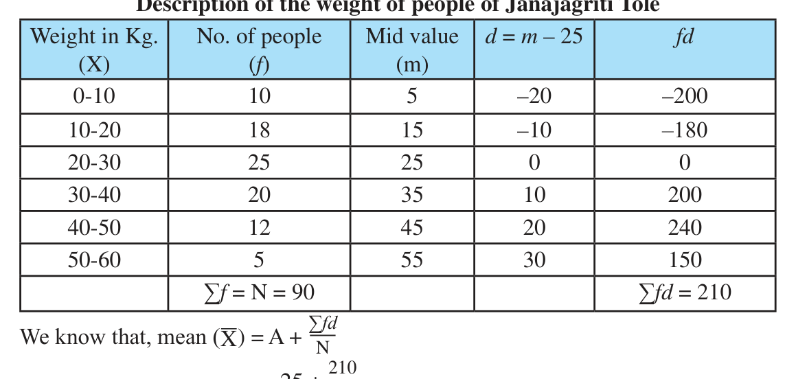
Step 1: The deviations from 25 are -20, -10, 0, 10, 20 and 30. Multiplying each by its frequency gives -200, -180, 0, 200, 240 and 150. Adding them:
\[ \sum fd = -200 - 180 + 0 + 200 + 240 + 150 = 210 \]
Step 2: Putting A = 25 and N = 90 into the formula:
\[ \overline{X} = 25 + \frac{210}{90} \]
Step 3: Dividing, then adding:
\[ \overline{X} = 25 + 2.33 = 27.33 \]
The mean weight of the people of the tole is 27.33 kg. Here Σfd is positive, so the mean is more than the assumed mean.
Finding a Missing Frequency
If the mean is known but one frequency is missing, give the missing frequency a letter and solve an equation. The mean height of the students of classes 11 and 12 of Shanti Secondary School is 157.75 cm. Their heights are grouped below, with one frequency written p. Find p.
| Height (cm) (X) | f | m | fm |
| 140-145 | 2 | 142.5 | 285 |
| 145-150 | 5 | 147.5 | 737.5 |
| 150-155 | 8 | 152.5 | 1220 |
| 155-160 | p | 157.5 | 157.5p |
| 160-165 | 7 | 162.5 | 1137.5 |
| 165-170 | 5 | 167.5 | 837.5 |
| 170-175 | 3 | 172.5 | 517.5 |
| Total | N = 30 + p | Σfm = 4735 + 157.5p |
Step 1: Adding the known frequencies and the known products, and keeping p as it is:
\[ N = 30 + p \]
\[ \sum fm = 4735 + 157.5p \]
Step 2: Putting the mean and the totals into the formula of the direct method:
\[ 157.75 = \frac{4735 + 157.5p}{30 + p} \]
Step 3: Multiplying both sides by (30 + p):
\[ 157.75(30 + p) = 4735 + 157.5p \]
Step 4: Opening the bracket on the left:
\[ 4732.5 + 157.75p = 4735 + 157.5p \]
Step 5: Taking the p terms to the left and the numbers to the right:
\[ 157.75p - 157.5p = 4735 - 4732.5 \]
Step 6: Simplifying both sides:
\[ 0.25p = 2.5 \]
Step 7: Dividing both sides by 0.25:
\[ p = 10 \]
Always check the answer. With \( p = 10 \), \( N = 40 \) and \( \sum fm = 4735 + 1575 = 6310 \). Then \( \frac{6310}{40} = 157.75 \), which is the mean we were given, so \( p = 10 \) is right.
Building the Frequency Table from Raw Data
The ages of the people who entered Balaju Park between 7 am and 8 am one morning were:
7, 22, 32, 47, 59, 16, 36, 17, 23, 39, 49, 31, 21, 24, 41, 12, 49, 21, 9, 8, 51, 36, 35, 18
Make a frequency table with a class interval of 10 and find the average age. The youngest person is 7 years old and the oldest is 59, so the classes 0-10, 10-20, 20-30, 30-40, 40-50 and 50-60 hold every age. Tallying each age into its class and counting the bars gives the frequencies:
| Age (years) (X) | Tally | f | m | fm |
| 0-10 | ||| | 3 | 5 | 15 |
| 10-20 | |||| | 4 | 15 | 60 |
| 20-30 | |||| crossed | 5 | 25 | 125 |
| 30-40 | |||| crossed, | | 6 | 35 | 210 |
| 40-50 | |||| | 4 | 45 | 180 |
| 50-60 | || | 2 | 55 | 110 |
| Total | N = 24 | Σfm = 700 |
Step 1: Adding the fm column:
\[ \sum fm = 15 + 60 + 125 + 210 + 180 + 110 = 700 \]
Step 2: Dividing by the number of people:
\[ \overline{X} = \frac{700}{24} \approx 29.17 \]
The average age of the people who visited the park in that hour is 29.17 years.
A mean has the same unit as the data it comes from. Write 29.17 years, 31.14 kg or 157.75 cm, never the bare number.
The full lesson is waiting for you
The notes are free to read in full. A free account opens the rest of the practice, and tracks your progress and confidence score for every subject. Presentations and videos need approval from Learn Yeti.