Seeing a Break in a Graph
Draw a graph without lifting your pencil from the paper and you get an unbroken curve. Some graphs cannot be drawn that way. Somewhere the pencil has to lift, because the curve has a gap, a hole or a sudden jump. Whether a graph is unbroken at a point is exactly what continuity is about. Compare the two graphs below.
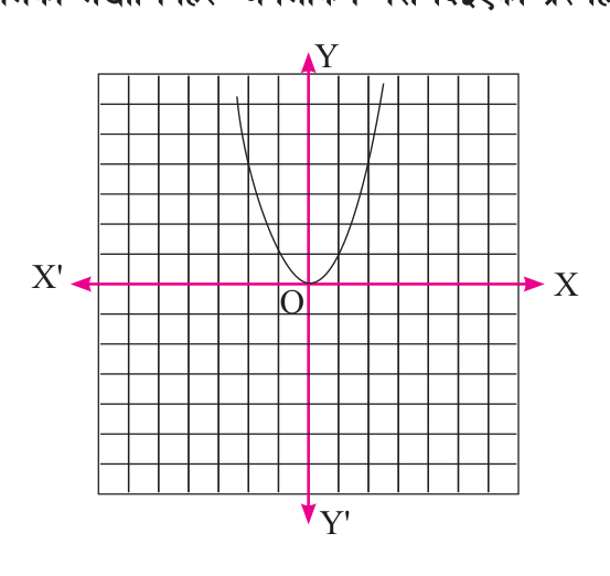
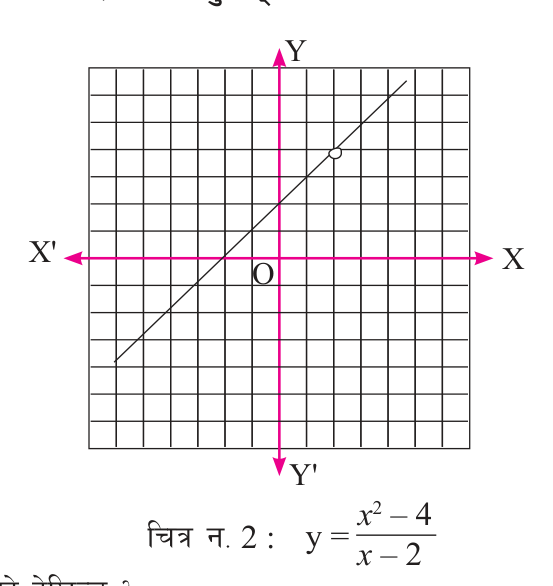
The first graph is \( y = x^2 \). It is a U-shaped curve with its lowest point at the origin, and it is not broken anywhere. Whatever point you choose on it, the curve runs smoothly into that point and out of it. We say this curve is continuous at every point, or continuous on the whole interval.
The second graph is \( y = \frac{x^2 - 4}{x - 2} \). It looks like an ordinary straight line, but at \( x = 2 \) there is a small empty circle. Put \( x = 2 \) into the formula and see what happens:
\[ y = \frac{2^2 - 4}{2 - 2} = \frac{0}{0} \]
The answer \( \frac{0}{0} \) is not a number, so there is no value of \( y \) at \( x = 2 \) and the point \( (2, y) \) cannot be plotted. The line has a hole there. At \( x = 2 \) this curve is discontinuous. At every other point it is continuous.
Continuous and discontinuous at a point: A curve is continuous at a point if it passes through that point without any break. It is discontinuous at a point if it has a break there, such as a hole, a gap or a jump.
A Road with a Hole
Picture three stretches of the same highway. On stretch A the road is smooth from start to end and never gives way. On stretch B there is a sharp V-shaped bend, but the road itself is not broken anywhere. On stretch C an earthquake has made the road collapse at exactly the 4 kilometre mark, \( x = 4 \), leaving a pit. Each stretch can be drawn as a graph, where \( x \) is the distance along the road and \( y = f(x) \) is the height of the road surface.
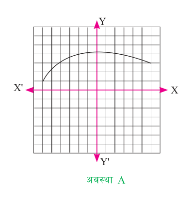
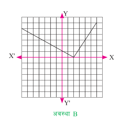
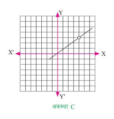
Road A is a continuous function. It runs on with no break at all. Road B is also a continuous function. The sharp corner changes the direction of the road, but a car can reach the bend and carry on without stopping. Road C is a discontinuous function, because at \( x = 4 \) the road has collapsed and a car cannot drive straight across the pit.
A sharp corner is not a break. A graph is discontinuous only where it has a hole, a gap or a jump.
Now study road C more closely. As \( x \) gets close to 4, the height of the road gets close to 3. We can check this with a table, walking towards \( x = 4 \) first from the left side and then from the right side.
| Direction | Value of x | Value of f(x) |
| From the left | 3.9 | 2.9 |
| From the left | 3.99 | 2.99 |
| From the left | 3.999 | 2.999 |
| At the point | 4 | no value (the pit) |
| From the right | 4.1 | 3.1 |
| From the right | 4.01 | 3.01 |
| From the right | 4.001 | 3.001 |
From the left, the heights 2.9, 2.99 and 2.999 creep up towards 3. From the right, the heights 3.1, 3.01 and 3.001 come down towards 3. Both sides are heading for the same height, which is 3.
Suppose the repair team fills the pit so that it meets the road surface exactly. That means giving the function a value at \( x = 4 \). Both sides of the road stand at height 3, so the filling must also reach height 3. Then \( f(4) = 3 \), the hole is gone and the road becomes continuous.
Left-Hand Limit and Right-Hand Limit
The value a function heads towards as \( x \) comes closer and closer to a point is called its limit at that point. Because \( x \) can approach a point from two sides, there are two one-sided limits.
Left-hand limit (LHL): The value that \( f(x) \) approaches as \( x \) comes closer to \( c \) through values less than \( c \). It is written \( \lim_{x \to c^-} f(x) \).
Right-hand limit (RHL): The value that \( f(x) \) approaches as \( x \) comes closer to \( c \) through values greater than \( c \). It is written \( \lim_{x \to c^+} f(x) \).
The symbol \( x \to 4^- \) is read as "x tends to 4 from the left", and \( x \to 4^+ \) as "x tends to 4 from the right". For road C, the table gives these two limits:
\[ \text{LHL} = \lim_{x \to 4^-} f(x) = 3 \]
\[ \text{RHL} = \lim_{x \to 4^+} f(x) = 3 \]
The small minus sign in \( 4^- \) does not mean negative numbers. It means approaching 4 from the smaller side, through values like 3.9, 3.99 and 3.999. In the same way, \( 4^+ \) means approaching through 4.1, 4.01 and 4.001.
When Does a Limit Exist?
A limit at a point exists only when the two sides agree about where the graph is heading.
Existence of a limit: The limit of \( f(x) \) at \( x = c \) exists when the left-hand limit and the right-hand limit are equal. Their common value is written \( \lim_{x \to c} f(x) \).
\[ \lim_{x \to c^-} f(x) = \lim_{x \to c^+} f(x) = L \]
For road C both one-sided limits are 3, so the limit exists and \( \lim_{x \to 4} f(x) = 3 \). If the two sides head for different heights, the graph jumps at \( c \), and then the limit does not exist at all.
Limit and Function Value Are Different Things
The limit tells us where the graph is heading as it approaches \( x = c \). The function value \( f(c) \) tells us where the graph actually is at \( x = c \). These two can be different, and one can exist without the other. Compare these two graphs.
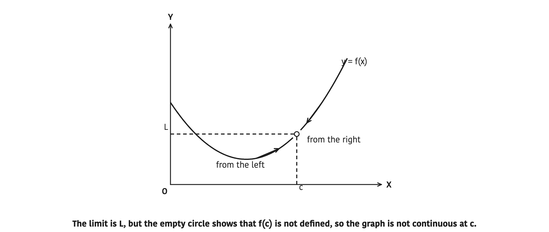
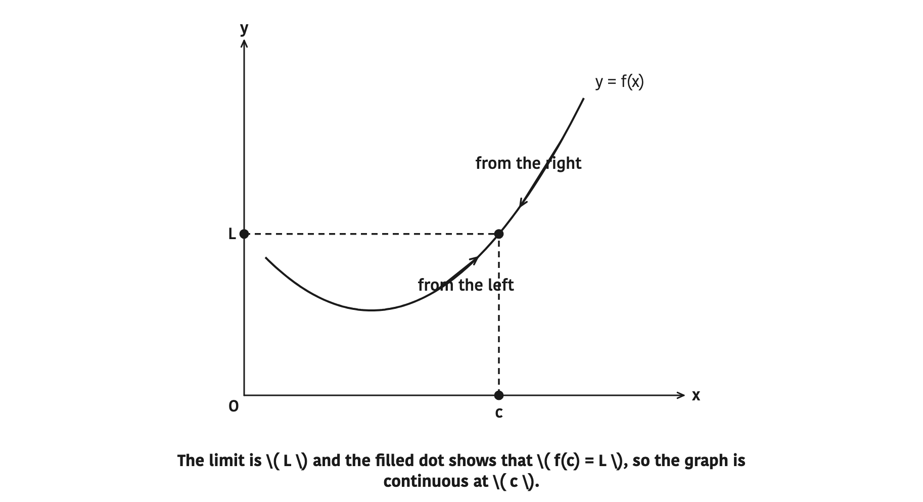
In both graphs the curve comes towards the same height \( L \) from the left and from the right, so in both graphs the limit exists and is equal to \( L \). In the first graph there is an empty circle at \( x = c \). An empty circle means the point is missing, so \( f(c) \) is not defined. In the second graph there is a filled dot at \( x = c \), which means the point is there and \( f(c) = L \). Only the second graph is continuous at \( x = c \).
Here is a question worth thinking about: if the limit exists, must the function value exist too? The first graph answers it. The limit exists, but \( f(c) \) does not. A limit alone is not enough for continuity.
An empty circle on a graph means the point is not included. A filled dot means it is included. Reading them the wrong way round turns a continuous graph into a discontinuous one.
Three Conditions for Continuity at a Point
Putting all of this together, a function \( f(x) \) is continuous at \( x = c \) only when all three of these conditions are true:
- 1. The limit \( \lim_{x \to c} f(x) \) exists. This means the left-hand limit equals the right-hand limit.
- 2. The function value \( f(c) \) is defined.
- 3. The limit and the function value are equal.
\[ \lim_{x \to c} f(x) = f(c) \]
Continuity at a point: A function \( f(x) \) is continuous at \( x = c \) if \( \lim_{x \to c^-} f(x) = \lim_{x \to c^+} f(x) = f(c) \).
Discontinuity at a point: A function is discontinuous at \( x = c \) if even one of the three conditions fails.
Continuous on an interval: A function is continuous on an interval if it is continuous at every point of that interval. Saying a curve is continuous from \( -4 \) to \( 4 \) means it has no break at any point between those two values.
How to Test Continuity at a Point
Every continuity question is worked in the same order. Keep these steps beside you while you study the examples that follow.
- Step 1: Find the left-hand limit, using values of x just less than c, or the rule of the function that applies to the left of c.
- Step 2: Find the right-hand limit, using values of x just greater than c, or the rule that applies to the right of c.
- Step 3: Compare the two. If they are different, the limit does not exist and the function is discontinuous, so you can stop here.
- Step 4: Find f(c) by putting x = c into the function. If this gives 0/0, or is undefined in any other way, the function is discontinuous.
- Step 5: If the limit and f(c) are equal, the function is continuous at x = c. If they are not equal, it is discontinuous.
Example 1: A Straight Line Function
Let \( f(x) = x + 1 \). Find \( f(x) \) when \( x = 1.9, 1.99, 1.999, 1.9999 \) and when \( x = 2.1, 2.01, 2.001, 2.0001 \). Then find \( f(2) \) and both one-sided limits at \( x = 2 \), and decide whether \( f(x) \) is continuous at \( x = 2 \).
Step 1: Putting values just less than 2 into \( f(x) = x + 1 \):
| x | f(x) = x + 1 |
| 1.9 | 1.9 + 1 = 2.9 |
| 1.99 | 1.99 + 1 = 2.99 |
| 1.999 | 1.999 + 1 = 2.999 |
| 1.9999 | 1.9999 + 1 = 2.9999 |
Step 2: Putting values just greater than 2 into the same function:
| x | f(x) = x + 1 |
| 2.1 | 2.1 + 1 = 3.1 |
| 2.01 | 2.01 + 1 = 3.01 |
| 2.001 | 2.001 + 1 = 3.001 |
| 2.0001 | 2.0001 + 1 = 3.0001 |
Step 3: Finding the value of the function at \( x = 2 \):
\[ f(2) = 2 + 1 = 3 \]
Step 4: Reading the left-hand limit from the first table, where the values rise towards 3:
\[ \lim_{x \to 2^-} f(x) = 3 \]
Step 5: Reading the right-hand limit from the second table, where the values fall towards 3:
\[ \lim_{x \to 2^+} f(x) = 3 \]
Step 6: Comparing all three values:
\[ \text{LHL} = \text{RHL} = f(2) = 3 \]
All three conditions hold, so \( f(x) = x + 1 \) is continuous at \( x = 2 \). Its graph is a straight line with no break.
Example 2: A Function Given in Two Pieces
Some functions follow one rule on one side of a point and a different rule on the other side. Such a function is called a piecewise function. Consider this one:
\[ f(x) = \begin{cases} x + 2, & 1 \le x \le 2 \\ 4x - 2, & x > 2 \end{cases} \]
Find \( f(1.99) \) and \( f(2.01) \), then find both one-sided limits at \( x = 2 \), and decide whether \( f(x) \) is continuous at \( x = 2 \).
Step 1: Since 1.99 lies between 1 and 2, the first rule \( f(x) = x + 2 \) applies:
\[ f(1.99) = 1.99 + 2 = 3.99 \]
Step 2: Since 2.01 is greater than 2, the second rule \( f(x) = 4x - 2 \) applies:
\[ f(2.01) = 4 \times 2.01 - 2 \]
\[ = 8.04 - 2 = 6.04 \]
Step 3: Finding the left-hand limit. To the left of 2 the rule is \( x + 2 \), and as \( x \) approaches 2 this approaches \( 2 + 2 \):
\[ \lim_{x \to 2^-} f(x) = 4 \]
Step 4: Finding the right-hand limit. To the right of 2 the rule is \( 4x - 2 \), which approaches \( 4 \times 2 - 2 \):
\[ \lim_{x \to 2^+} f(x) = 6 \]
Step 5: Comparing the two one-sided limits:
\[ \lim_{x \to 2^-} f(x) \neq \lim_{x \to 2^+} f(x) \]
The two sides head for different heights, 4 and 6, so the limit at \( x = 2 \) does not exist. The first condition fails, and \( f(x) \) is not continuous at \( x = 2 \). Notice that \( f(2) = 2 + 2 = 4 \) is defined, yet this does not help: once the two sides disagree, the function is discontinuous whatever \( f(2) \) is. On a graph, the curve reaches height 4 at \( x = 2 \) and then jumps up to start again from height 6.
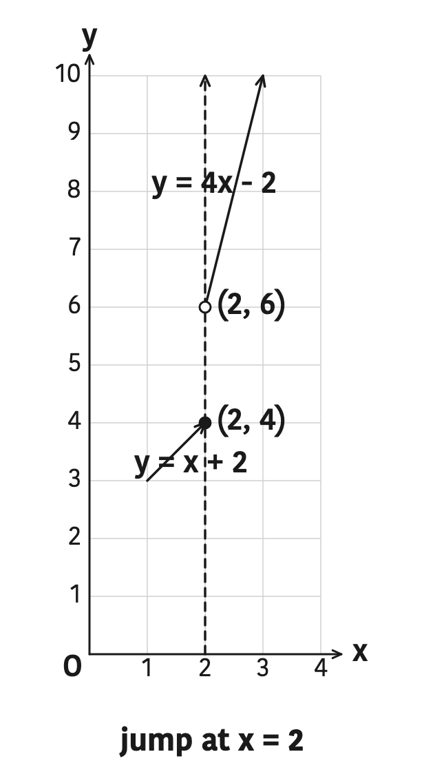
For a piecewise function, the left-hand limit comes from the rule on the left of the point and the right-hand limit comes from the rule on the right. The point where the rule changes is the point to test.
Example 3: A Function That Gives Zero by Zero
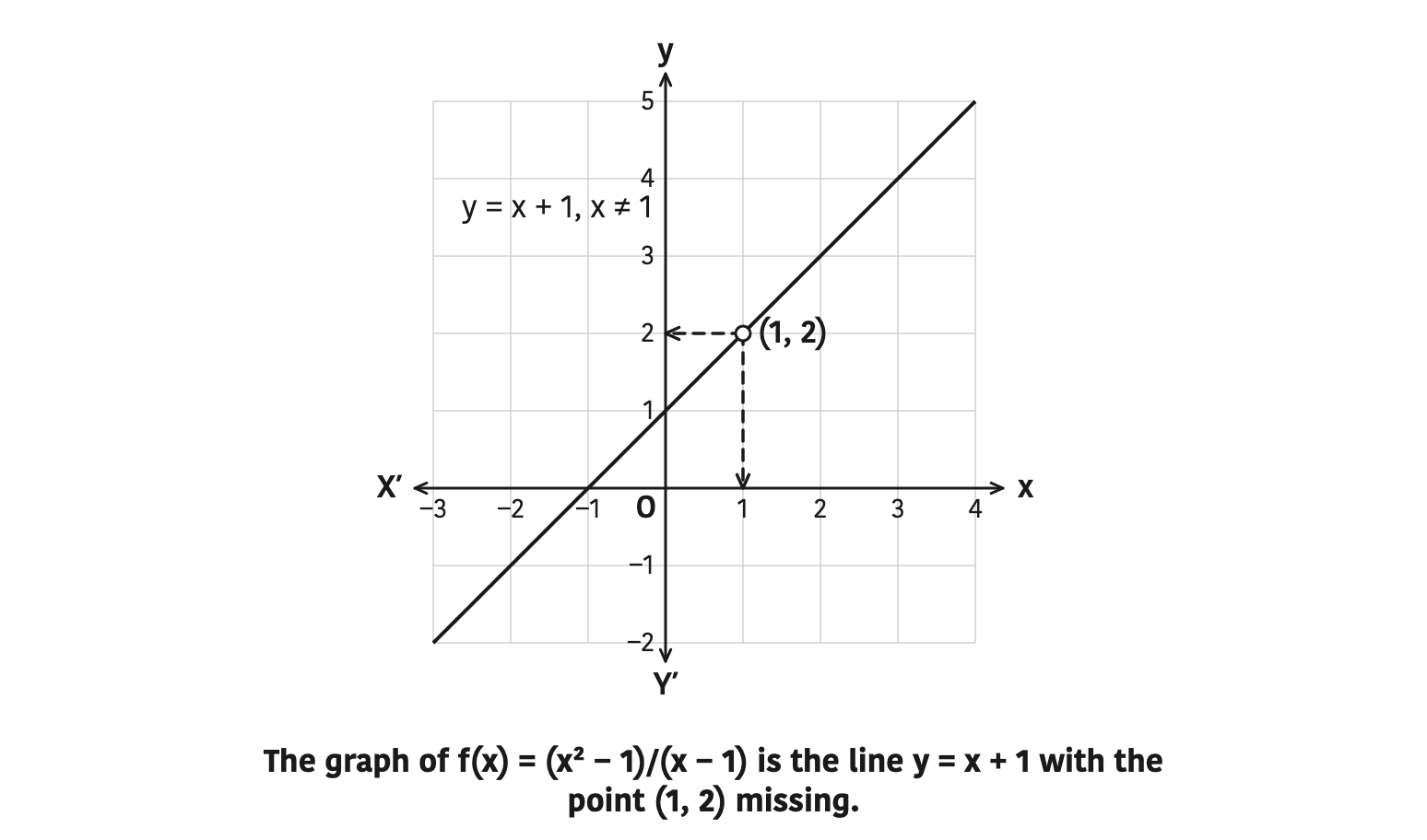
Test the continuity of \( f(x) = \frac{x^2 - 1}{x - 1} \) at \( x = 1 \) by putting in values of \( x \) close to 1.
Step 1: Writing down what continuity at \( x = 1 \) needs, which is the limit equal to the function value:
\[ \lim_{x \to 1} f(x) = f(1) \]
Step 2: Putting values of \( x \) very close to 1, from the left and from the right, into \( f(x) \):
| x (from the left) | f(x) | x (from the right) | f(x) |
| 0.9 | 1.9 | 1.1 | 2.1 |
| 0.99 | 1.99 | 1.01 | 2.01 |
| 0.999 | 1.999 | 1.001 | 2.001 |
| 0.9999 | 1.9999 | 1.0001 | 2.0001 |
Step 3: Reading the table. From either side, as \( x \) gets closer to 1, \( f(x) \) gets closer to 2, so the limit is:
\[ \lim_{x \to 1} f(x) = 2 \]
Step 4: Finding the function value by putting \( x = 1 \) into the function:
\[ f(1) = \frac{1^2 - 1}{1 - 1} = \frac{0}{0} \]
The result \( \frac{0}{0} \) is an indeterminate form, so \( f(1) \) is not defined. The limit exists and equals 2, but the actual value of the function at \( x = 1 \) does not exist.
Indeterminate form: An expression such as \( \frac{0}{0} \) that has no definite value. When substituting a value of \( x \) gives \( \frac{0}{0} \), the function is not defined at that point.
Step 5: Comparing the limit with the function value:
\[ \lim_{x \to 1} f(x) \neq f(1) \]
So the function is discontinuous at \( x = 1 \). The table values make sense once you factorise: \( \frac{(x - 1)(x + 1)}{x - 1} = x + 1 \) for every \( x \neq 1 \). The graph is therefore the line \( y = x + 1 \) with one point missing, the point \( (1, 2) \).
\( \frac{0}{0} \) is not 0 and it is not 1. It has no value at all. Writing \( f(1) = 0 \) or \( f(1) = 1 \) here is wrong.
Example 4: Proving a Function Is Not Continuous
Prove that \( f(x) = \frac{x^2 + x - 6}{x + 3} \) is not continuous at \( x = -3 \).
Step 1: To make the table easy to fill in, factorise the numerator. Since \( x^2 + x - 6 = (x - 2)(x + 3) \), the function becomes:
\[ f(x) = \frac{(x - 2)(x + 3)}{x + 3} \]
Step 2: Cancelling the common factor \( x + 3 \). This is allowed only while \( x \neq -3 \), because at \( x = -3 \) we would be dividing by zero:
\[ f(x) = x - 2, \quad x \neq -3 \]
Step 3: Putting values of \( x \) close to \( -3 \) into \( x - 2 \):
| x (from the left) | f(x) = x - 2 | x (from the right) | f(x) = x - 2 |
| -3.1 | -5.1 | -2.9 | -4.9 |
| -3.01 | -5.01 | -2.99 | -4.99 |
| -3.001 | -5.001 | -2.999 | -4.999 |
| -3.0001 | -5.0001 | -2.9999 | -4.9999 |
Step 4: Reading the table. As \( x \to -3 \) from either side, \( f(x) \to -5 \), so:
\[ \lim_{x \to -3} f(x) = -5 \]
Step 5: Finding the function value by putting \( x = -3 \) into the original function:
\[ f(-3) = \frac{(-3)^2 + (-3) - 6}{-3 + 3} \]
Step 6: Simplifying the top and the bottom:
\[ f(-3) = \frac{9 - 3 - 6}{0} = \frac{0}{0} \]
This is the indeterminate form, so \( f(-3) \) is not defined. The limit exists and equals \( -5 \), but the function value at \( x = -3 \) does not exist. The second condition fails, so \( f(x) \) is not continuous at \( x = -3 \), which is what we had to prove.
Cancelling \( x + 3 \) is how we find the limit. It does not give the value at \( x = -3 \). To find \( f(-3) \), always substitute into the original function.
The full lesson is waiting for you
The notes are free to read in full. A free account opens the rest of the practice, and tracks your progress and confidence score for every subject. Presentations and videos need approval from Learn Yeti.